Gmail Survival Analysis

An introduction to gmailr, the KM-estimator, and Cox models

I’m on a mission to incorporate survival analysis into as many areas of my life as possible. Last year, I used Kaplan-Meier plots to track progress in my job search. This year, I decided to tackle my inbox. Eager to graduate from tweeting about survival analysis to blogging about it, I’ve written up a guide to how you can access and model your own email data.

Parsing Old Emails with gmailr

gmailr is a simple way to access your own Gmail data in R. Jenny Bryan has written a great tutorial on how to send emails with the package, but I couldn’t find a lot of documentation on how to parse sent emails. I’m hoping to fill that gap with a mini-tutorial of my own.

There are two main functions for searching your email: messages() and threads(). messages() returns a list of messages that match your query, while threads() includes all emails in any thread that matches the query.

In our case, we’re interested in getting all sent emails and figuring out whether we got a response. Messages in the sent folder only includes emails written by me, so to figure out whether the recipient responded we need to search for threads.

all_threads <- threads('in:sent')

The messages themselves are stored in the messages object.

message_details <- lapply(all_threads, '[[', 'messages')

gmailr comes with various utility functions for extracting details from the message, such as body(), subject(), date(), to(), and from(). These will return strings extracted from the Gmail MIME object, and depending on what you’re trying to do you might have to format them further.

The to and from fields can have different formatting depending on the email. I wrote a helper function to strip all names and only return sorted and lowercase email addresses, making it easy to match recipient across email threads.

parse_email <- function(field) {
    if( grepl('<', field) ) {
        components <- sort( stringr::str_extract_all(field, '<[^<>]+>')[[1]] );
        parsed.field <- paste(components, collapse = ',')
    } else {
        parsed.field <- field
    }
    return( tolower( gsub('<|>', '', parsed.field) ) )
}

Another messy part is extracting the message itself. When people hit reply to your email, the response will typically look something like this:

Message example

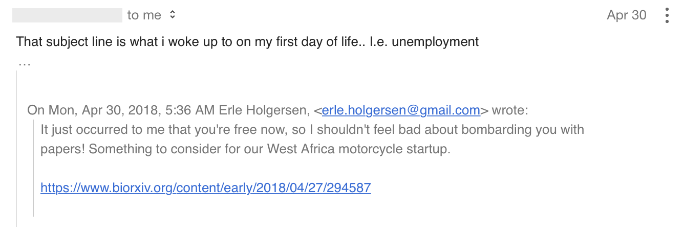
Calling body() on this message will return everything, including “Erle Holgersen, <erle.holgersen@gmail.com> wrote:” and my original email.

To separate out only the most recent part of the conversation, I kept only the parts before the first “@” or “wrote:”. The approach is obviously imperfect, but it’s a quick way to get something that should at least resemble an email.

There was one further complication. The body() function only works for multipart messages, which excludes some particularly short emails. In those cases I opted to use the short snippet object as the email text instead.

# store data as we go along
all_details <- list()

# loop over messages in thread
for( m in message_details ) {

    full_text <- body(m)
    if( length(full_text) > 0 ) {
        last_message <- strsplit(full_text[[1]][1], split = paste0('@|wrote:'))[[1]][1]
    } else {
        last_message <- m$snippet
    }
            
    all_details[[ m$id ]] <- data.frame(
        thread_id = thread_id,
        message_id = m$id,
        from = parse_email( from(m) ),
        to = parse_email( to(m) ),
        date = strptime(date(m), format = '%a, %d %b %Y %H:%M:%S %z'),
        subject = ifelse(!is.null( subject(m) ), subject(m), ''),
        message = last_message
    );
}

all_details <- do.call(rbind, all_details)

At this point, I also did a factor relevelling exercise to protect my own privacy. Instead of keeping all of the original email addresses, I changed all but my own into a random name from the randomNames package. With everyone’s identities hidden, we can start looking at who I’ve been emailing.

In total I sent 2,849 emails over the period to a total of 289 different recipients. 78% of the emails were addressed to one of the 25 most frequently contacted people, and almost a third to Allyson.

Top recipients

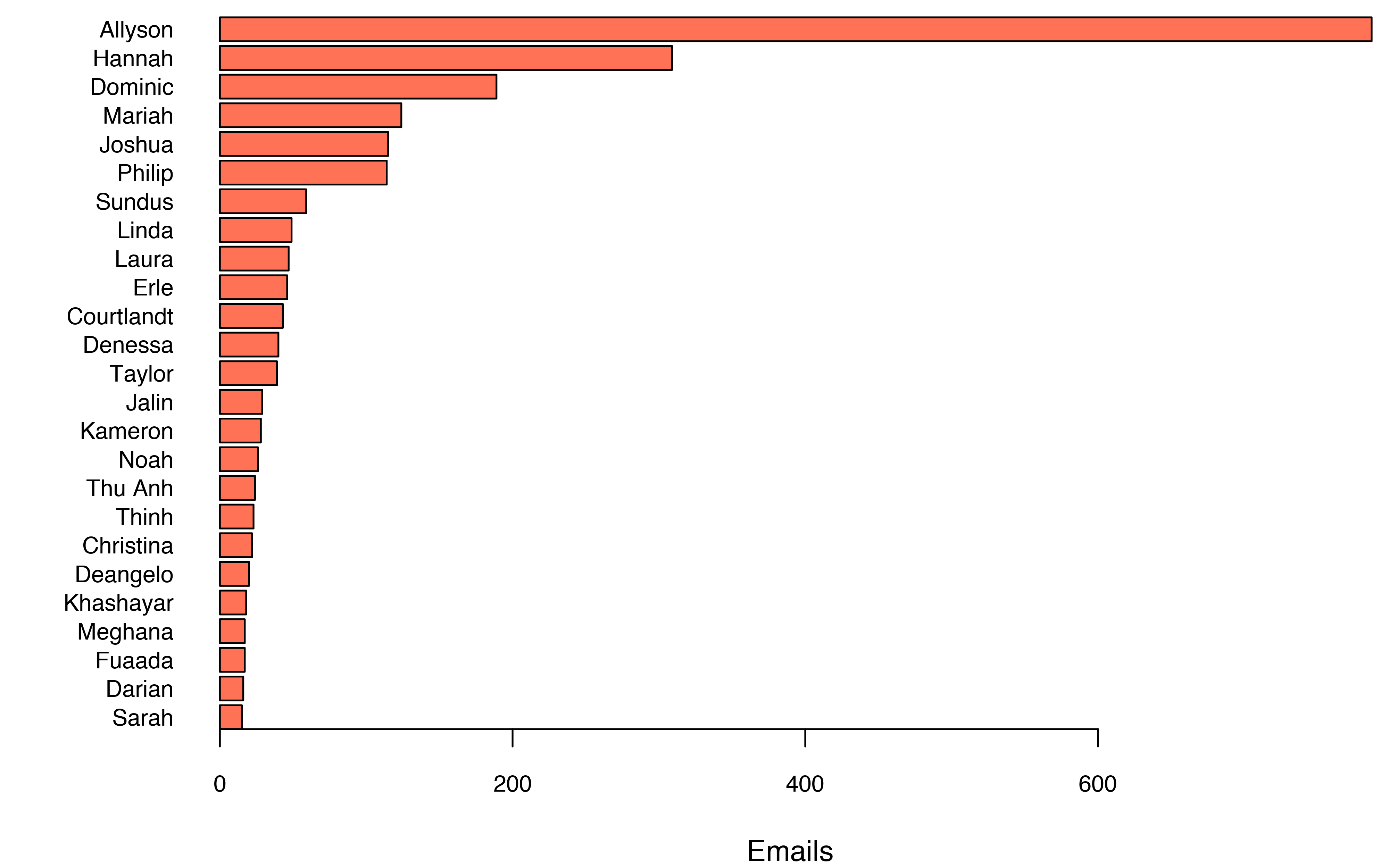
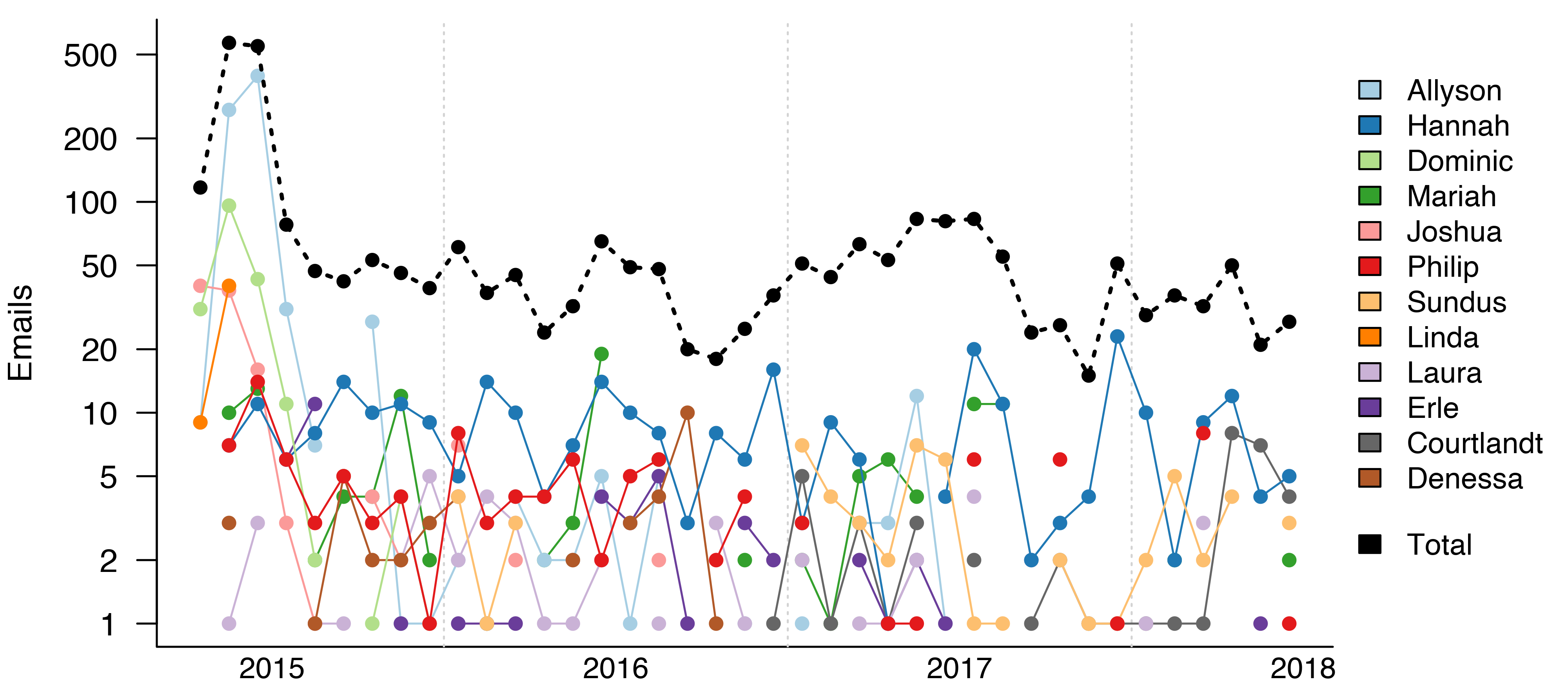
If you look carefully at the graph, you’ll see I’m my own 10th most frequent email target. I mostly send myself attachment-only emails, but there are some other use cases too. For example, the most recent self-email I sent was the result of Jenny Bryan’s gmailr tutorial.

Self-emails

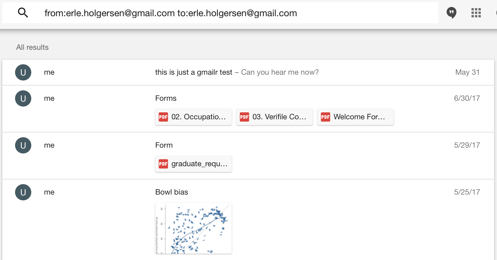
Of course, three years is a long time, and I haven’t been emailing everyone at the same rate. Most of my emails to Allyson and Dominic were sent in the summer of 2015¹. By contrast, I have been consistently emailing Hannah at a rate of around 10 emails a month for the past three years.

Self-emails

Reformatting for Survival Analysis

So far we’ve parsed all of my email messages and focused on the ones I’ve sent. To do survival analysis we need to reformat this data to get the time to response for every email.

Even though it’s called survival analysis, we use the term to refer to any analysis of time-to-event data. For example, it’s commonly used in clinical trials to analyze time to progression on a particular treatment. The same techniques can also be used on very different datasets, like analyzing how long it takes website users to complete a form.

A defining feature of this kind of data is censoring. In clinical trials, some patients’ disease might never progress. Even though we don’t have a survival time for them, we still need to include these observations in the data to avoid biasing the analysis.

For my Gmail data, censored observations are emails that went unanswered. There are two ways this can happen:

1. I sent an email and never heard back
2. I sent an email, grew impatient, and sent a follow-up email

In the second case, the other person might eventually get back to me, but there’s no way of knowing when they would have responded if I hadn’t nagged them. To include information about the email they didn’t answer for X days, I consider the original email as censored on the day I sent a follow-up message.

km_data <- list()

for(thread_data in split(all_details, all_details$thread_id) ) {
    thread_id <- thread_data$thread_id[1]
    
    # order by date of email
    thread_data <- thread_data[ order(thread_data$date), ]
    
    last_sent <- grepl(my_email, thread_data$from[1])
    last_date <- thread_data$date[1]
    
    # loop over messages to add survival information
    if( nrow(thread_data) > 1 ) {
        for(i in 2:nrow(thread_data) ) {
            new_date <- thread_data$date[i]
            new_sent <- grepl(my_email, thread_data$from[i])
            
            if( last_sent ) {
                km_data[[ paste0(thread_id, '_', as.character(i)) ]] <- data.frame(
                    date = last_date,
                    time = as.numeric(difftime(new_date, last_date, units = 'days')),
                    to = thread_data$to[i-1],
                    reply = !new_sent, # consider as censored if I've sent follow-up
                    subject = thread_data$subject[i-1],
                    message = thread_data$message[i-1]
                    )
            }
            last_date <- new_date
            last_sent <- new_sent
        }
    }
    
    # if the last message in the thread was from me,
    # add it as a censored observation at the current date
    if( last_sent ) {
        km_data[[ paste0(thread_id, '_final') ]] <- data.frame(
            date = last_date,
            time = as.numeric(difftime(Sys.time(), last_date, units = 'days')),
            to = thread_data$to[ nrow(thread_data) ],
            reply = FALSE,
            subject = thread_data$subject[ nrow(thread_data) ],
            message = thread_data$message[ nrow(thread_data) ]
            )
    }
}

Visualization: The Kaplan-Meier Estimator

There are two ubiquitous tools in survival analysis: the Kaplan-Meier estimator and Cox proportional hazards model. I’m going to briefly explain each of them here, and show how they can be applied to my email data.

The Kaplan-Meier estimator is a non-parametric estimator of the survival rate. It was first published in 1958, and if you’ve ever read a paper in a medical journal, you’re likely to have seen it in action.

Here’s an example from a paper published by my division recently (Tutt et al., 2018):

TNT trial

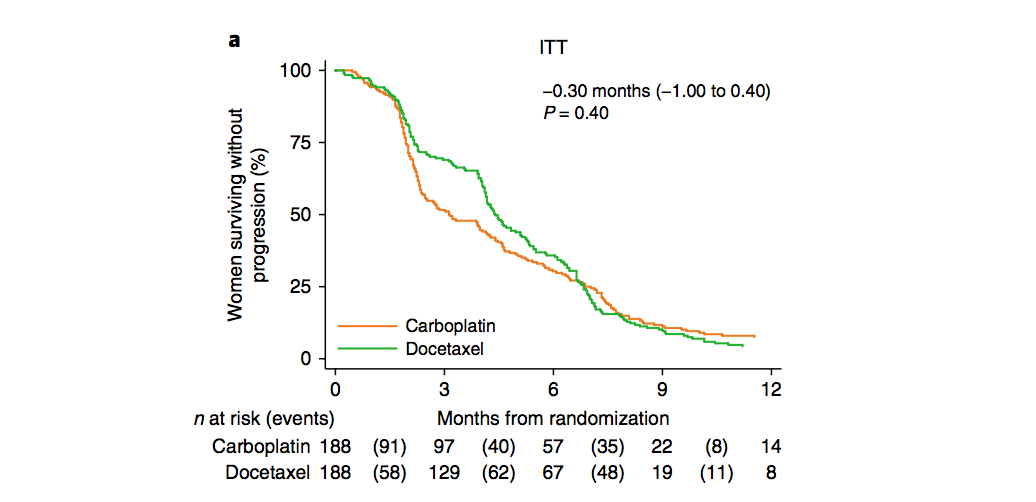
The Tripe-Negative Trial compared two types of chemotherapy in patients with triple-negative or BRCA-deficient breast cancer. The plot shows the proportion of patients in each treatment group whose cancer still hadn’t progressed after a certain number of months.

Mathematically, the Kaplan-Meier estimator at time \(t\) is a product over all event times \(t_i \leq t\).

\[\begin{equation} \hat{S}(t) = \prod_{i: t_i\leq t} \left( 1 - \frac{d_i}{n_i}\right) \end{equation}\]

where \(d_i\) is the number of events at time \(t_i\) (e.g. the number of patients who died), and \(n_i\) is the number of events that could have happened at time \(t_i\). This is typically the number of patients who were known to be alive just prior to \(t_i\), and is referred to as the number “at risk.”

In R, the survival package is the most common way of calculating and plotting the Kaplan-Meier estimator. If we run survfit without any predictors, we get a visualization of the overall response rate. The plus signs represent censored observations.

survfit_object <- survfit(Surv(time, reply) ~ 1, km_data);
plot(
    survfit_object,
    mark.time = TRUE,
    xlim = c(0, 14),
    conf.int = FALSE,
    xlab = 'Days since email',
    ylab = 'Response-free rate',
    lwd = 2
    ) 

Overall KM plot

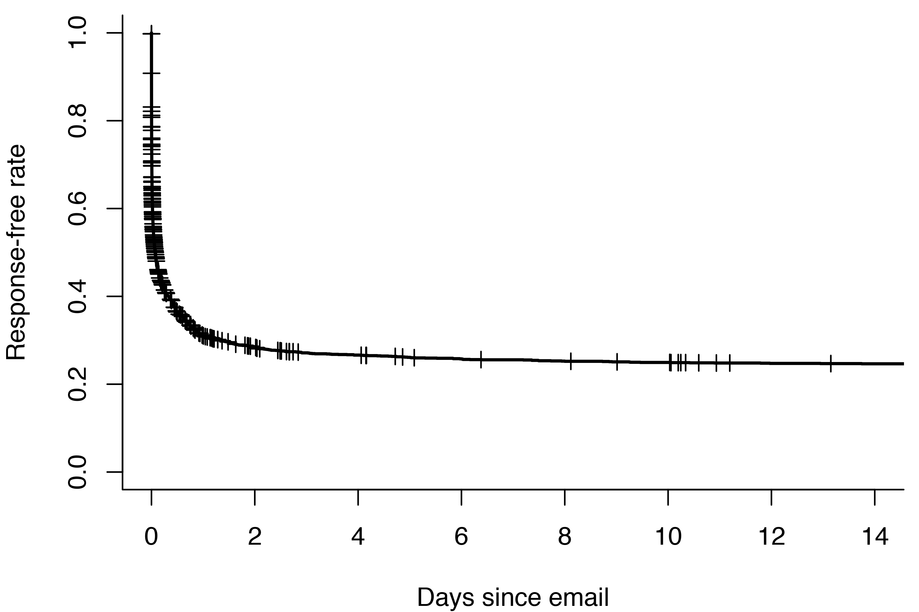
Over 70% of the emails I send get a response within two weeks. Better than I feared! But as you might expect, not everyone I email is equally dedicated to responding to me. The 20-day response rate of my top 12 most used contacts varies between zero and 93%.

Person KM plot

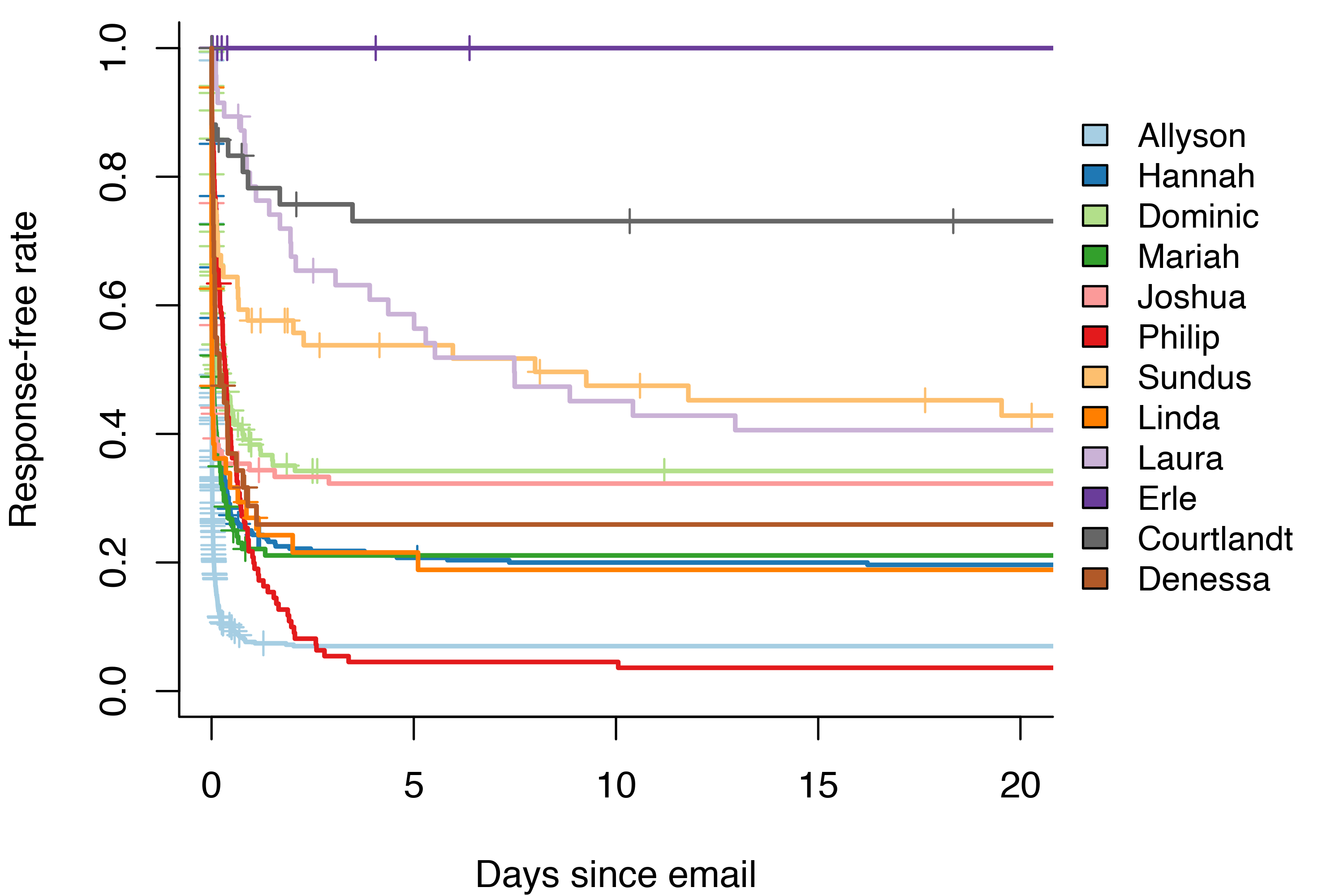
Thankfully, the response rate of zero is not quite as bad as it seems. I’m my own least dedicated email responder. Due to the way I counted emails as censored, any time there was more than one email in a thread between me and me, it would still count as a censored observation rather than a response. Oh well.

Out of all of the other people I email, Courtlandt has the worst response rate at 27%. At the other end of the spectrum we have Allyson and Philip, who respond to over 90% of my emails.

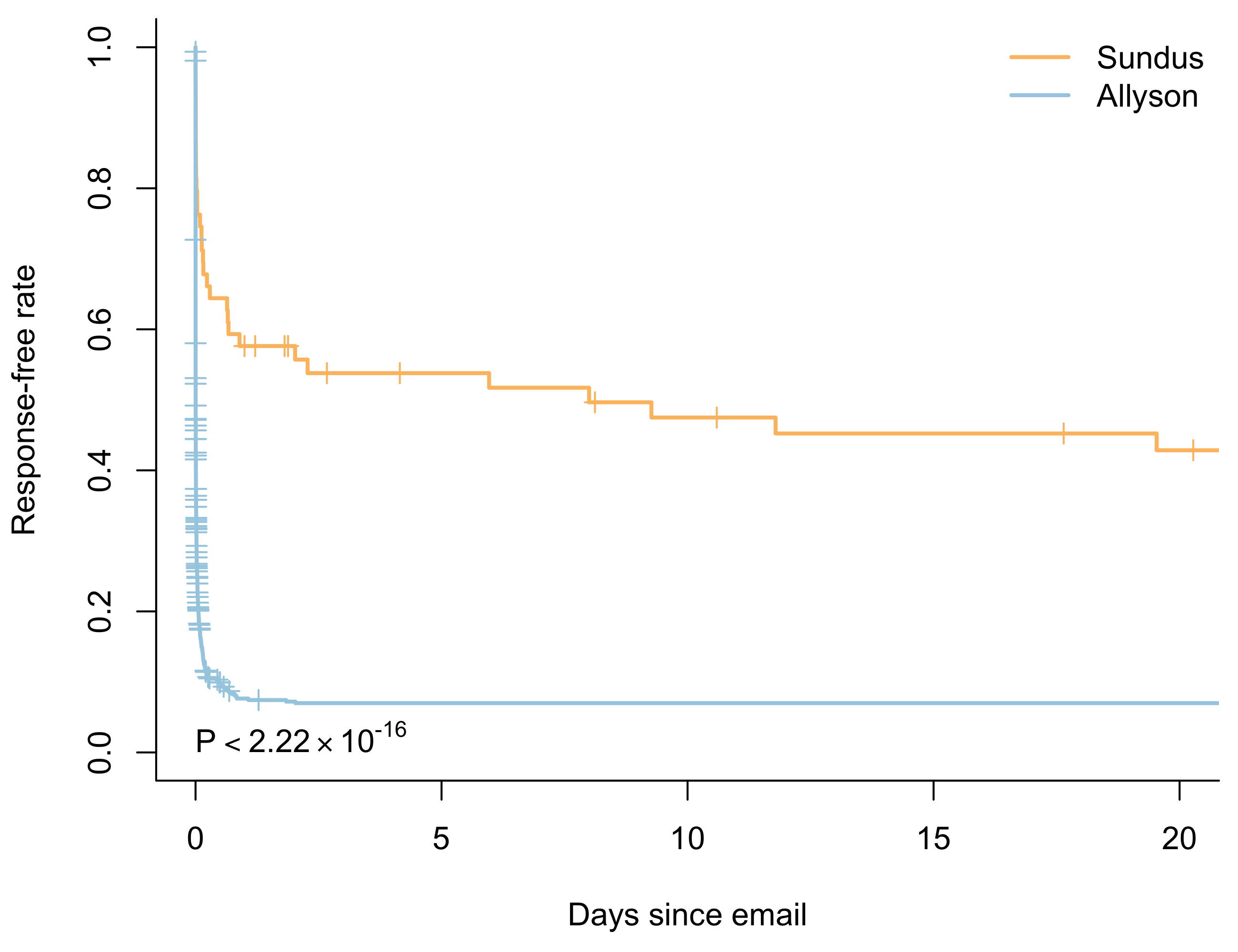
Interestingly, most people seem to respond to my email within two days – if they’re going to respond at all. Two exceptions are Sundus and Laura. Laura responds at a roughly steady rate for the first 10 days. On the other hand, Sundus responds to 40% of my emails within 18 hours. She then continues to respond at a much slower rate for the next 20 days, perhaps reflecting some underlying mixture distribution.

This idea that events happen at different rates at different times is key to another concept in survival analysis: the hazard function.

The hazard function \(\lambda(t)\) is the instantaneous rate of events at time \(t\).

\[\begin{equation} \lambda(t) = \lim_{dt \to 0} \frac{Pr\left( t \leq T < t + dt | T \geq t \right)}{dt} \end{equation}\]

The numerator gives the conditional probability of an event happening between \(t\) and \(dt\), given that no event had happened by \(t\). By taking the limit as \(dt\) goes to zero, we get the rate at which events happen at time \(t\).

Modelling: Cox Proportional Hazards

The most common way of fitting regression models to survival data makes heavy use of the hazard function. In 1972, Cox published a semi-parametric model for survival data called the proportional hazards model.

Like the name suggestions, the “proportional hazards” model assumes that the hazard function for two groups is proportional. Take for example Allyson and Courtlandt. Under the proportional hazards assumption, we assume that Courtlandt’s hazard function \(\lambda_C(t)\) is a constant multiple of Allyson’s hazard function \(\lambda_A(t)\).

\[\begin{equation} \frac{\lambda\_{\text{A}}(t)}{\lambda\_{\text{C}}(t)} = K \;\; \text{for all times}\;\; t \end{equation}\]

In more mathematical terms, we can write the hazard function at time \(t\) for an individual with covariates \(X_i\) as

\[\begin{equation} \lambda(t \mid X_i)= \lambda\_0(t) \exp(\beta X_i) \end{equation}\]

The beauty of this approach is that we’re able to estimate the coefficient vector \(\beta\) without ever specifying the baseline hazard \(\lambda\_0(t)\). The estimation is accomplished by maximizing the partial likelihood.

When changing a single predictor \(x_j\), the relationship between the two hazard functions \(e^{\beta_j}\) is known as the hazard ratio. We can estimate it with the coxph() function in the survival package.

people <- c('Courtlandt', 'Allyson');

courtlandt_allyson <- km_data %>%
    filter(to %in% people) %>%
    mutate(to = factor(to, levels = people));

cox_model <- coxph(Surv(time, reply) ~ to, courtlandt_allyson);

> print( summary(cox_model) )
Call:
coxph(formula = Surv(time, reply) ~ to, data = courtlandt_allyson)

  n= 830, number of events= 673 

            coef exp(coef) se(coef)    z Pr(>|z|)    
toAllyson 2.2153    9.1639   0.3064 7.23 4.84e-13 ***
---
Signif. codes:  0 ‘***’ 0.001 ‘**’ 0.01 ‘*’ 0.05 ‘.’ 0.1 ‘ ’ 1

          exp(coef) exp(-coef) lower .95 upper .95
toAllyson     9.164     0.1091     5.027     16.71

Concordance= 0.539  (se = 0.006 )
Rsquare= 0.127   (max possible= 1 )
Likelihood ratio test= 112.4  on 1 df,   p=0
Wald test            = 52.27  on 1 df,   p=4.835e-13
Score (logrank) test = 75.86  on 1 df,   p=0

The exp(coef) column gives the hazard ratio. In the case of comparing Allyson’s response rate to Courtlandt’s, it’s 9.16. If I send the same email to both of them and wait for a response, in any given moment the estimated probability of Allyson responding is almost 10 times greater than the probability of Courtlandt responding!

Courtlandt/ Allyson KM plot

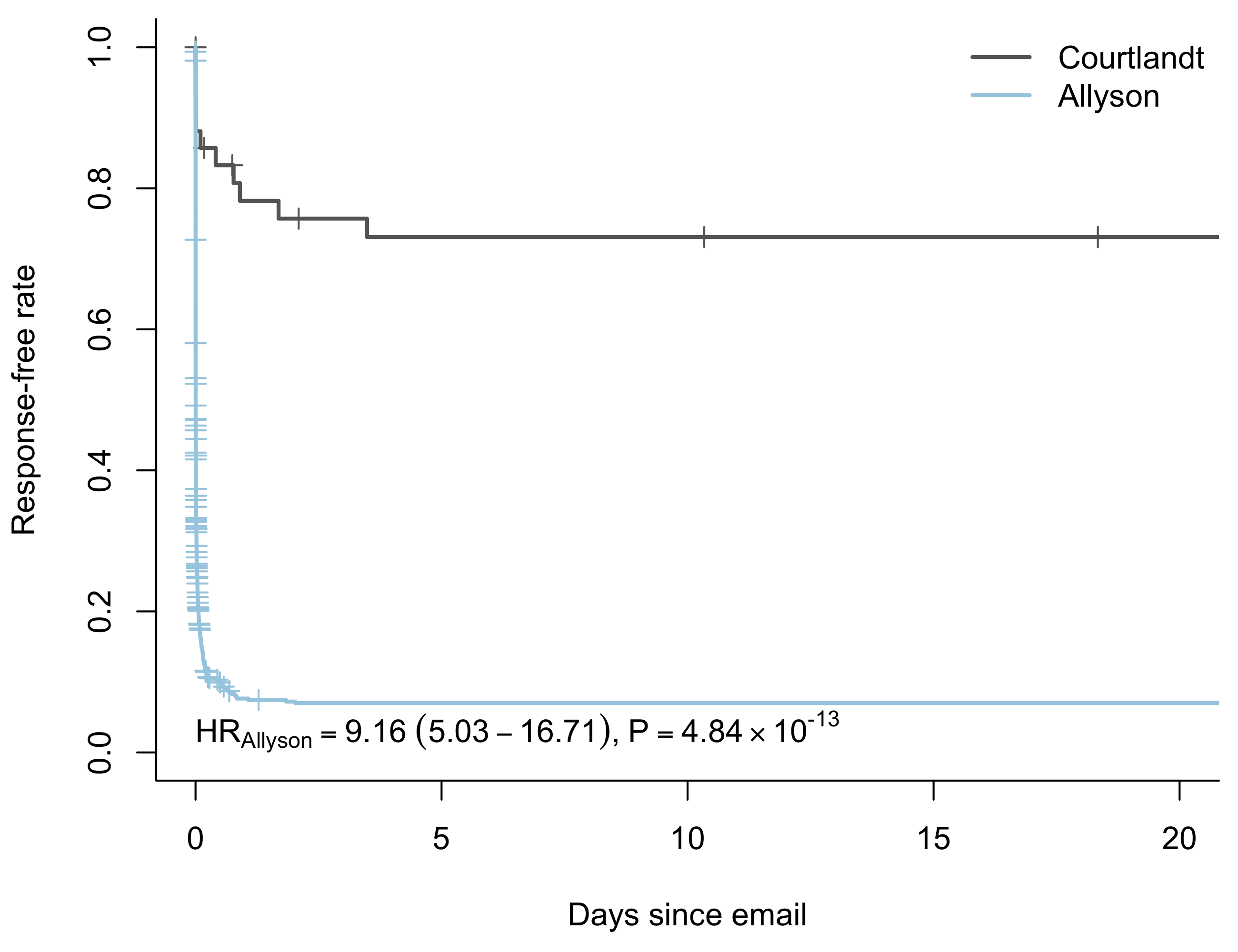
Does the proportional hazards assumption always hold? Of course not. To make sure our parameter estimates are valid, we have to check that the assumption holds. The cox.zph() function in the survival package makes that easy.

> print(cox.zph(cox_model))
              rho chisq     p
toAllyson -0.0325 0.689 0.406

In this case, the test of the proportional hazards assumption returns a \(p\)-value of 0.406. There’s no evidence to reject the assumption, and our proportional hazards model is most likely reasonable.

What about Sundus with the response time mixture distribution? Is her hazard function still proportional to Allyson’s? Not surprisingly, it isn’t. We reject the null hypothesis of proportional hazards with a \(p\)-value of 0.0018. If we want to model the relationship between Allyson’s and Sundus’ response times we have to look to alternative techniques such as the logrank test.

Sundus/ Allyson KM plot

The Cox proportional hazards model also has one weapon against non-proportional hazards: stratification. If we’re not primarily interested in the differences between recipients, but would still like to include an adjustment term in a multivariate model, we can use stratification.

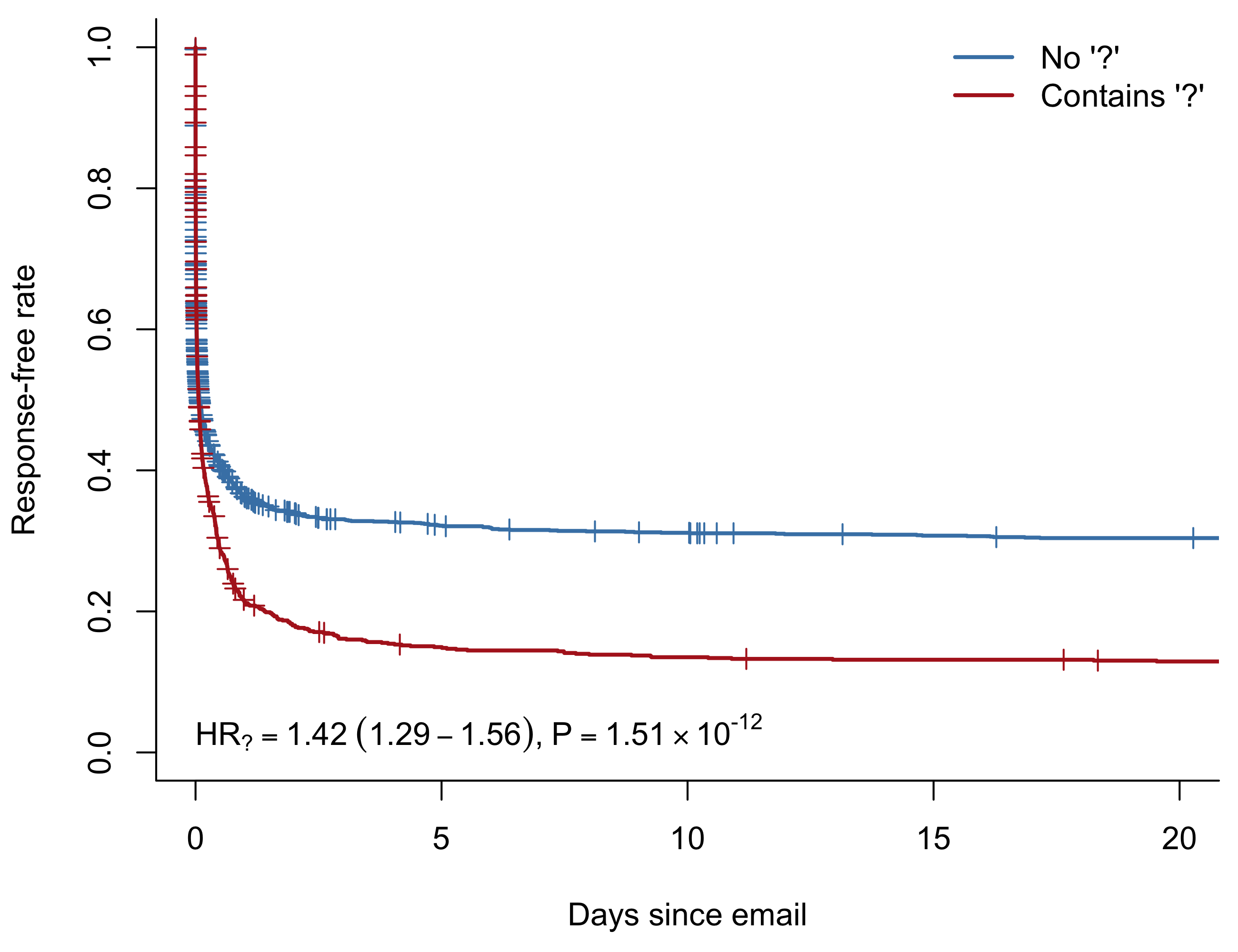
For example, consider my tweet about asking questions. It’s possible that such a model could be confounded by the recipient. If I tend to send more questions to people who have higher response rates anyways, this could lead to a significant question mark effect that would not generalize to a new cohort.

To test whether this might be the case, we can fit a new model stratifying on recipient. The stratification allows for the baseline hazard to be different for each individual. We still estimate the hazard ratio for including a question mark across all recipients, but we’re no longer limited by the proportional hazards assumption between individuals.

question_mark <- grepl('\\?', km_data$message)
cox_model <- coxph(
    Surv(time, reply) ~ strata(to) + question_mark, 
    km_data
    )

There’s no way of showing the stratification in a KM plot, but we can overlay the hazard ratio and \(p\)-value from the stratified model to give a more accurate picture of the effect.

Stratified question KM

I also extended this analysis to look at other frequently used terms/ characters such as smiley faces and exclamation marks.

predictors <- list(
    '?' = grepl('\\?', km_data$message),
    ':D' = grepl(':D', km_data$message),
    ':)' = grepl(':)', km_data$message),
    ':P' = grepl(':P', km_data$message),
    '!' = grepl('\\!', km_data$message),
    'http' = grepl('http', km_data$message),
    'Erle' = grepl('Erle', km_data$message)
    )

combined_hrs <- list()
for(predictor_name in names(predictors)) {
    predictor <- predictors[[ predictor_name ]]
    cox_model <- coxph(
        Surv(time, reply) ~ sxtrata(to) + predictor, 
        km_data
        )
    combined_hrs[[ predictor_name ]] <- broom::tidy(cox_model)
}

The forest plot shows the confidence intervals for the coefficient \(\beta_j\) in each of these models.

Forest plot

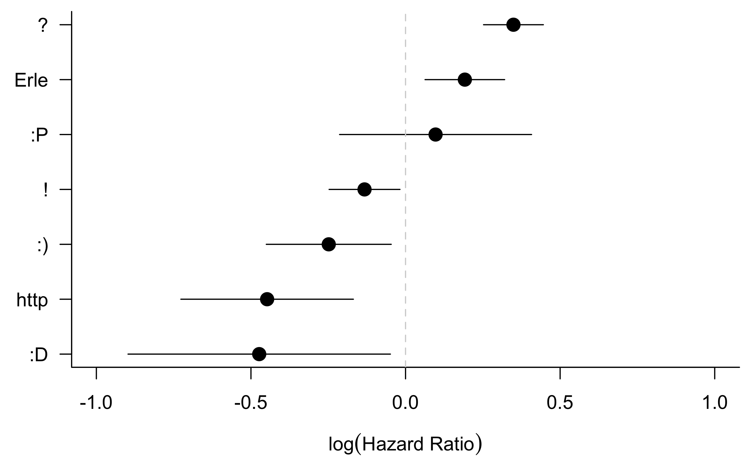
Including a question or a proper sign-off in an email seems to improve the response time. By contrast, including more “fun” things such as exclamation marks, moderately happy, and very happy smiley faces makes people slower to respond. Links also appear to be an unpopular addition to emails.

Conclusion

There’s a lot more to survival analysis than what I’ve covered here. When I first started this project I planned to try and build a multivariate predictive model for email response. Then I realized that this post is already approaching 3,000 words, and I’m better off leaving it for another time – but I’d still like to highlight two particularly relevant techniques.

Cure models are an extension of survival models that allow for “cured” individuals. Traditionally, we assume that every subject would experience the event of interest if we waited long enough. This makes sense when looking at survival: everyone dies eventually. But as we all know, some emails go permanently unanswered.

Another option would be to use a recurrent event model. For the purposes of this post I have conveniently ignored the fact that sometimes I’m the one who doesn’t respond. People might have to send me several emails to follow up, giving me recurrent event data I could try modelling. Maybe next time!

Footnotes

1. If you’re worried about what happened to Allyson, I can assure you we still keep in touch – by text.