Adjusting for batch effects in the Star Wars trilogies
Star Wars and batch effects came into my life around the same time. Back in late 2016, I went through a few months of intense interest in both. I was finishing up an internship in cancer genomics, and at one point it seemed like every project I worked on was plagued by batch effects.
Batch effects are technical sources of variation that cause problems with genomics experiments. Wet lab biology is finicky. As a general rule, changing anything will lead to different results. New reagent? Batch effect. New person preparing the samples? Probably also a batch effect.
At the single gene level, a batch effect might look like a slight difference in the average expression.
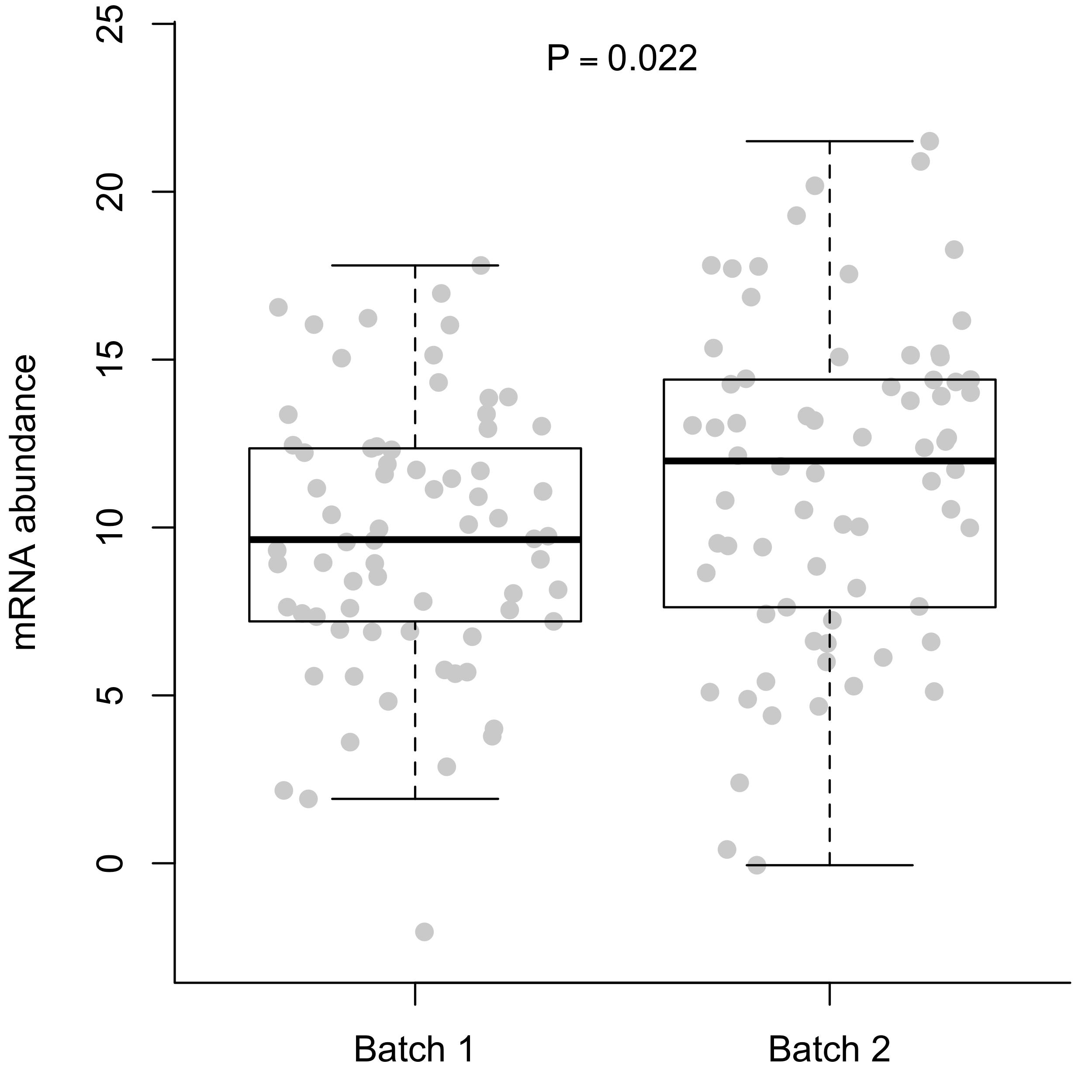
Differences are typically more pronounced when you combine all of the genes. If you plot the first two principal components, it’s not uncommon to end up with complete separation of the batches.
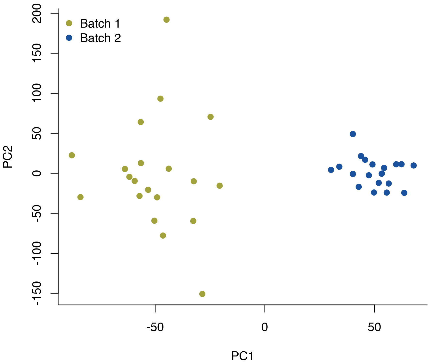
These batch effects can make it difficult to compare across groups of samples that weren’t processed in exactly the same way. For example, if the groups you’re interested in comparing aren’t evenly split across the batches, it can be difficult to disentangle any group differences from the batch effect. The problem has sparked a lot of research into statistical methods for adjusting for batch effects, and there are various R packages and other tools available.
Around the same time I was struggling with this, I made plans to go see Rogue One with one of my coworkers. And of course it struck me: the Star Wars movies were done in batches! Batch effects had infiltrated both my professional and personal lives. Ever since this realization, I’ve wanted to treat Star Wars like a microarray dataset and run a batch-correction method.
Data Collection
Not quite at the level of working with video data, I opted to use screenshots as input for the batch correction. Theoretically speaking, you could consider every frame as a separate screenshot and use all of them as input. In practice, that’s far too much data for my computer to deal with. To reduce the computational requirements, I only took one screenshot every minute.
I wrote an AppleScript to automate the screenshot-process. AppleScript is a lot like English, and with the help of Google I was able to write a script that did exactly what I wanted, despite not having any experience with the language.
set video to "PATH_TO_VIDEO"

tell application "VLC" to activate
    tell application "VLC" to open video

    tell application "VLC"
        set elapsed to current time
        set tMax to duration of current item
    end tell

    repeat while elapsed < tMax
        tell application "VLC"
            repeat 6 times
                step forward
            end repeat
            set elapsed to current time
        end tell
        tell application "System Events"
            keystroke "s" using {command down, option down}
        end tell
    end repeat
To keep things simple, I excluded the most recent (in progress) batch of movies from the analysis. I ran the code above for each of the six movies in the original and prequel trilogies, leaving me with 653 screenshots in total.
Reading the Screenshots in R
The imager package is a quick way to get started with image data in R. On a boring, data-storage level, an image is a three-dimensional array. The first two dimensions are the x- and y-coordinates of the pixel, and the third dimension gives the colour. With RGB colours, this third dimension has length three, corresponding to red, green, and blue colour intensity.
For example, a 2x1 pixel image can be stored as a data frame with six rows. The value column contains the colour intensity, and the other three columns specify the coordinates.
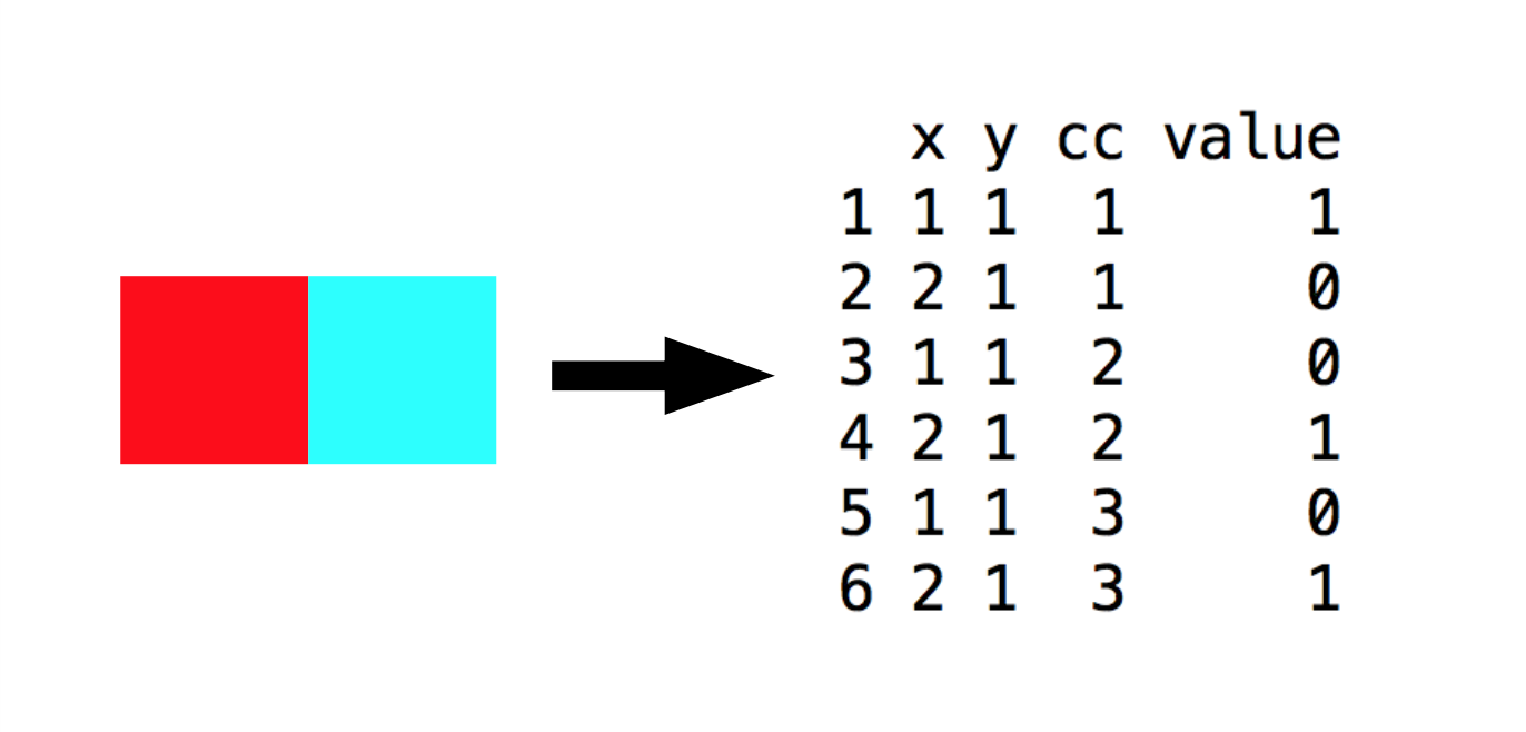
I read each Star Wars screenshot into R with the load.image() function, converted it to a data frame, and extracted the value column. The coordinates are the same for every screenshot, allowing me to reduce my data down to a matrix where each row corresponded to the value column for a particular screenshot.
To make my life easier, I made two additional tweaks. First, I re-sized the images to a quarter of their original size. With every pixel being stored three times, downsizing makes a huge difference for both speed and memory.
Secondly, I applied a logit transformation to the pixel intensities. Statistics is generally easier when you have unbounded values, and all of my data fell in the range \([0, 1]\). The logit transform allowed me to run the batch correction without worrying too much about the distribution assumptions.1
\[\begin{equation} y' = \text{logit}(y) = \log \left( \frac{y}{1-y} \right) \end{equation}\]
In the end, this data processing left me with a 653x293,760 matrix of screenshots X and a vector Y giving the batch for each screenshot.
Testing for Batch Effects
Before adjusting for batch effects, it’s generally a good idea to check if there are any. There are two main ways of doing this:
- Run a dimensionality reduction method (e.g. PCA) to visually check if the batches cluster together
- Test for differences in each pixel (or gene, if you’re a genomics person)
In my case, visualizing the data in two dimensions did not show any evidence for batch effects. When plotting each screenshot by the first two principal components, the two trilogies overlap almost perfectly.
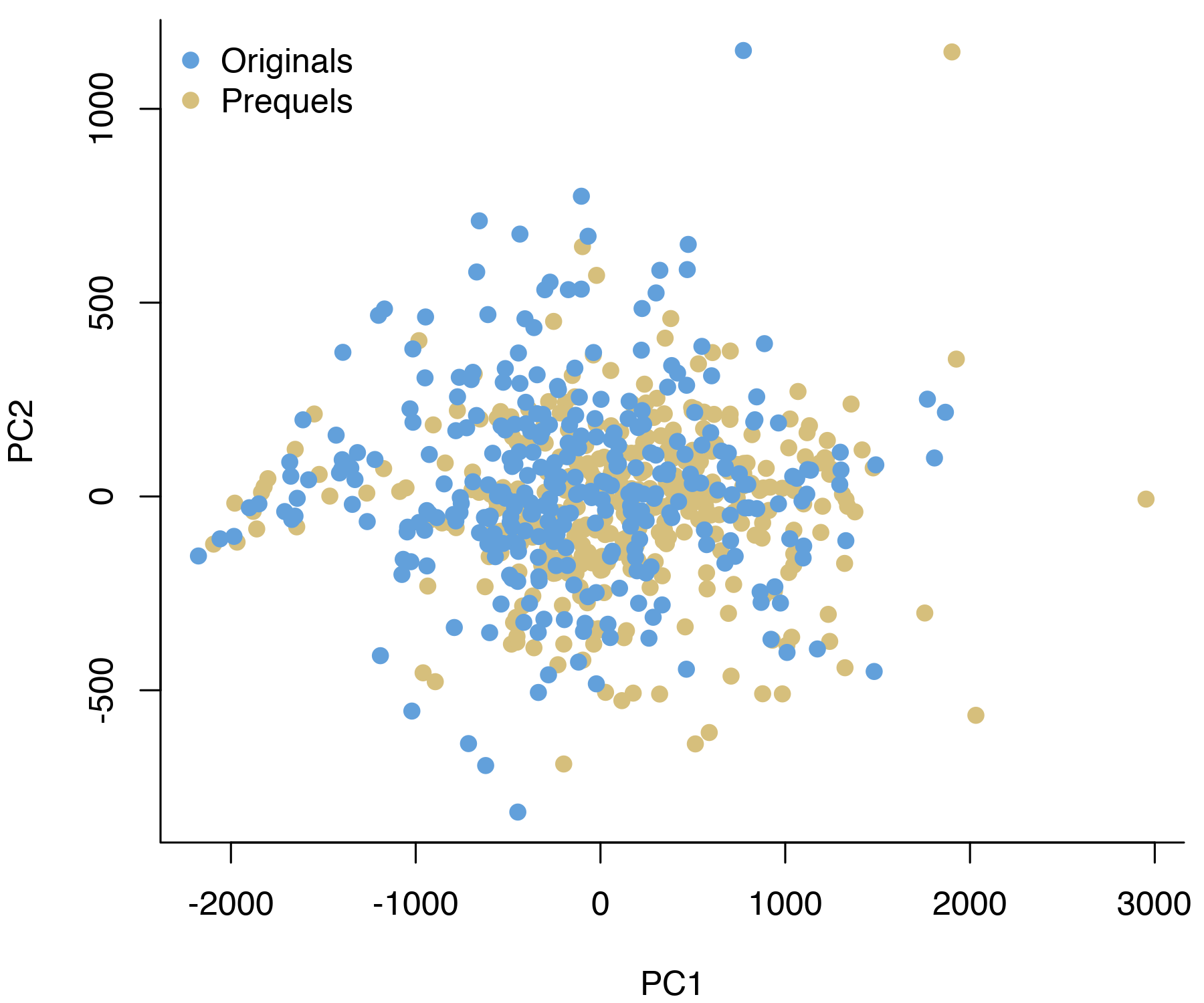
Of course, the lack of clear batch effects in this plot doesn’t mean we don’t have to worry about them. As a more formal test, I ran a t-test for differences in intensity of each colour channel for every pixel. By plotting the resulting \(p\)-values, we can quickly get a sense for whether there are differences between the batches. If the null hypothesis (no difference between the trilogies) is true for every pixel, we’d expect the \(p\)-values to be uniformly distributed.
In our case, the \(p\)-values are anything but uniform.
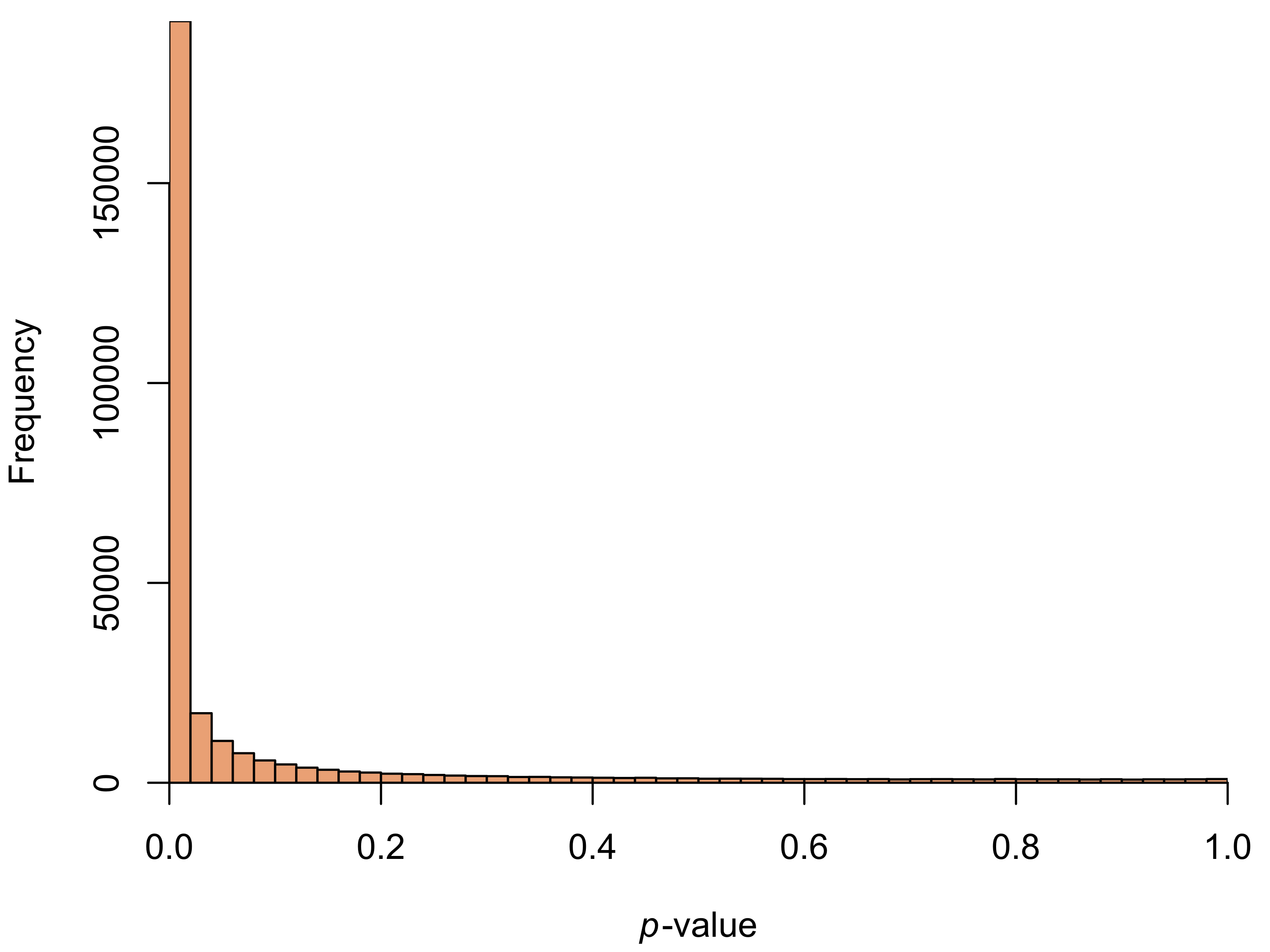
David Robinson has a great post on interpreting \(p\)-value histograms. Our histogram is a prime example of what he calls the “Hooray!” type: the large number of small \(p\)-values means we reject the null hypothesis for a large number of tests.2
In ordinary genomics studies, we’d typically stop here. The histogram shows that there is a batch effect, and we can proceed to adjust for it. However, this being my first experience with imaging data, I wanted to try and interpret the batch differences more visually.
The simplest way to visualize the differences is to consider the difference in average pixel colour. For each colour channel of each pixel, I averaged over all screenshots in the batch to create an “average screenshot” from each trilogy.
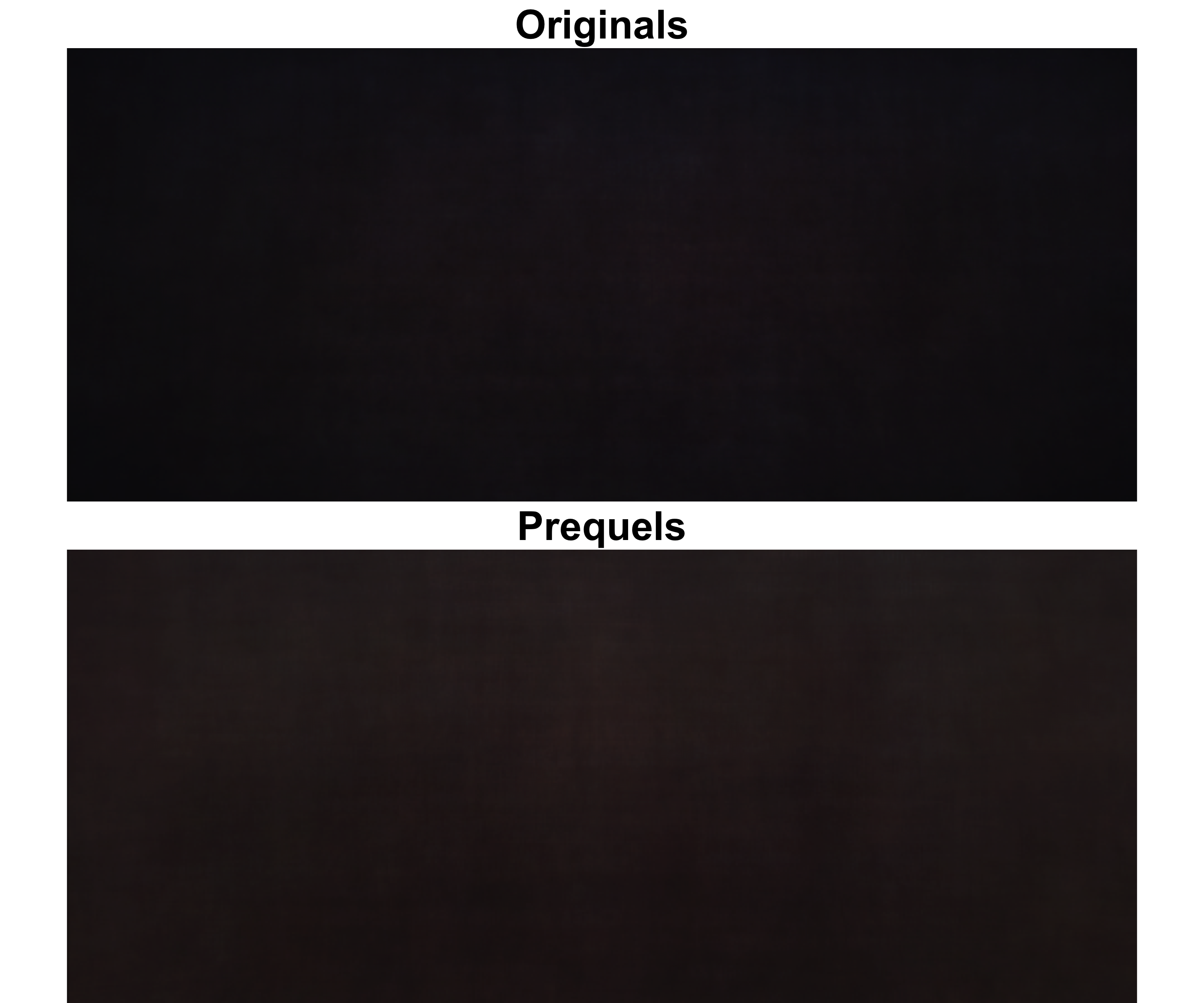
Not surprisingly, these average screenshots are boring. But they do give us some sense of the batch effect: the prequel screenshots seem to have lighter, more brown-ish colours. This is also clear from the \(t\)-tests: all of the tests with a \(p\)-value less than 0.05 had a higher pixel intensity in the prequels than the original trilogies.
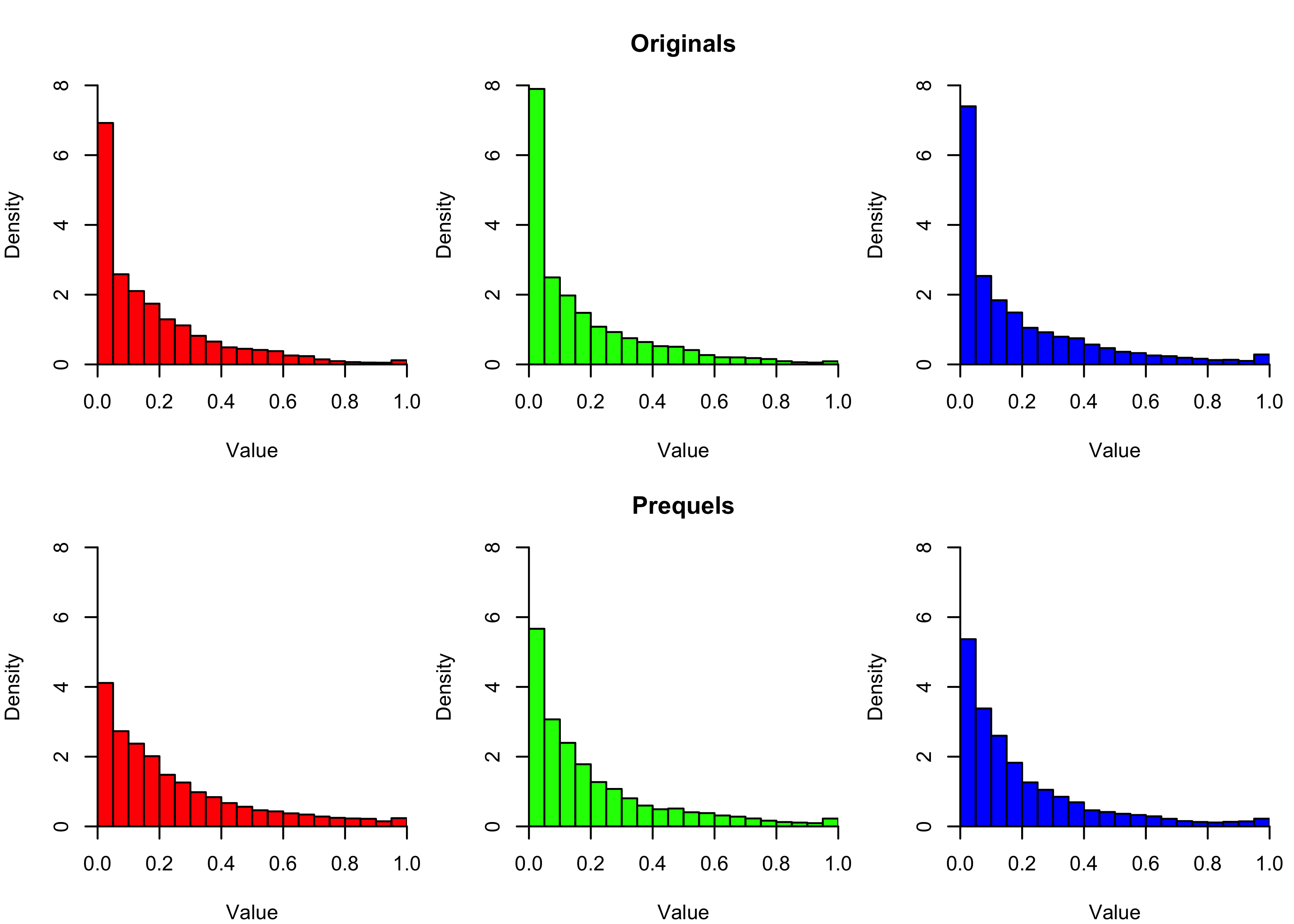
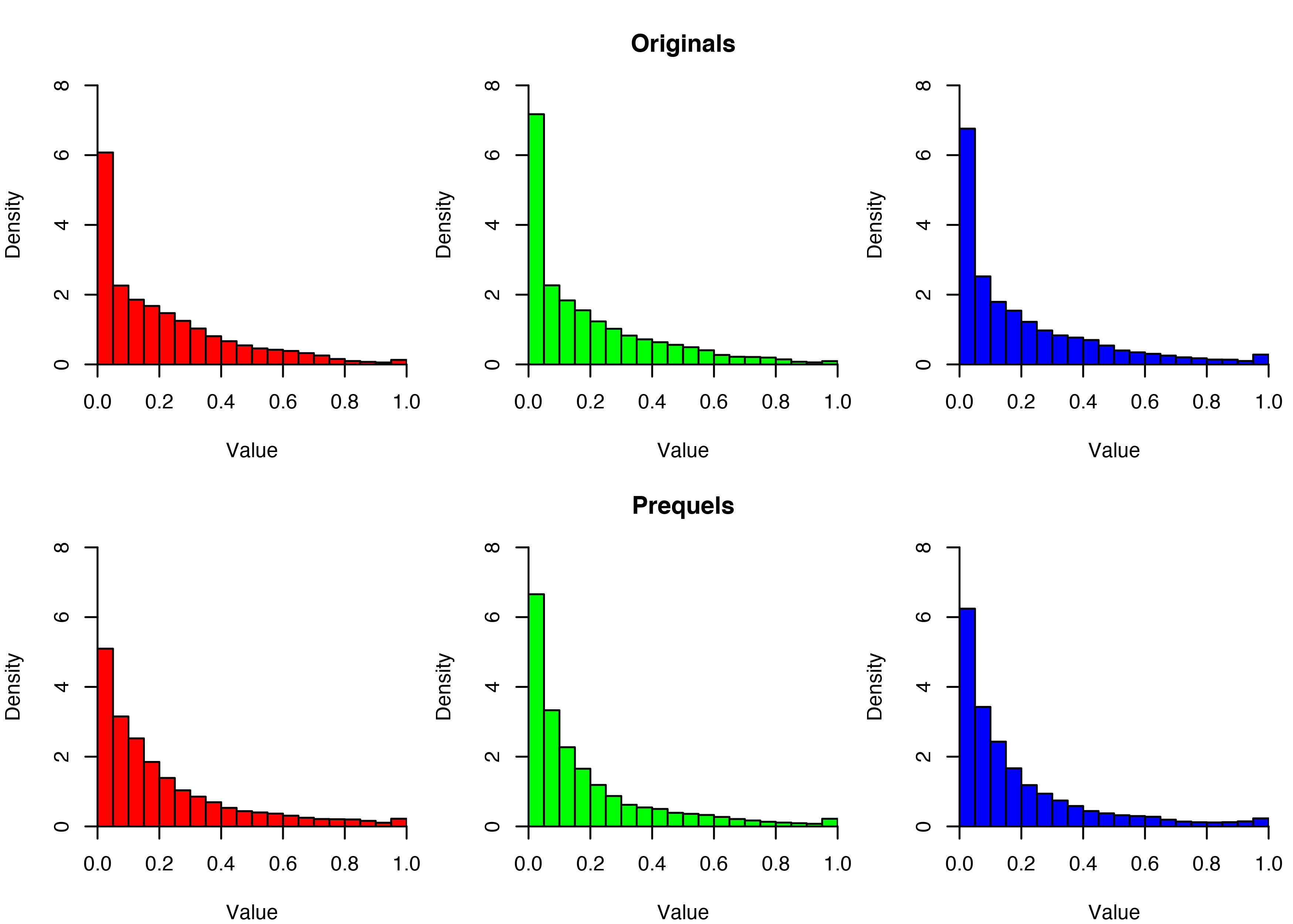
We can dig further into this by separating out the colour channels. The histograms below show the intensity values of each colour channel for each trilogy. Consistent with the average screenshots above, we see near-zero intensities are more common in the originals than the prequels.
Another way of visualizing the differences is through the spatial arrangement of the differential intensity pixels. I considered the three colour channels separately, and plotted all pixels with a significant batch effect.

The differential intensity pixels seem to be concentrated towards the edges of the screen. For all channels there’s a set of unaffected pixels in the middle (shown in white). This area is considerably smaller for the red and green channels than the blue one, which could indicate that the prequels use warmer colours than the original movies.
The corner effect becomes even clearer when you merge the colour channels and plot any pixel with a batch effect in any channel. Increasing the significance threshold clearly shows that the pixels closer to the edge of the screen have larger batch effects than the ones in the center.

In photography terms, dark corners is known as vignetting. It can happen either due to poor lens quality, or be applied as a cinematographic effect to draw the viewer’s attention to the center of the frame. I don’t know enough about cinema to say what’s the case here, but it seems clear that the original trilogy has more vignetting than the prequels.
Running ComBat
To perform the actual batch-adjustment, I ran ComBat. The method was first published in 2007, and takes an empirical Bayes approach.
All Bayesian methods need a prior distribution for the data. For empirical Bayes methods, we use the dataset as a whole to estimate the prior distribution. When estimating the batch effects for our Star Wars dataset, this means we’re borrowing strength across all of the pixels. If the pixel intensities tend to be higher in one trilogy than the other, we incorporate that information into every pixel-specific estimate.3
In mathematical terms, this involves a lot of Greek letters. Assume that the intensity of the \(p\)th pixel in batch \(i\) is given by
\[\begin{equation} Y_{ijp} = \alpha_p + X\beta_p + \gamma_{ip} + \delta_{ip}\epsilon_{ijp} \end{equation}\]
where \(\alpha_p\) is the average intensity of the pixel, \(X\) is the model matrix, \(\beta_p\) is a vector of coefficients for the covariates, \(\gamma_{ip}\) is the additive batch effect, \(\delta_{ip}\) is the multiplicative batch effect, and \(\epsilon_{ijp} \sim N(0, \sigma^2_p)\) is an error term.
The ComBat method involves three steps. First, the model parameters \(\hat{\alpha}_p\), \(\hat{\beta}_p\), and \(\hat{\gamma}_{ip}\) are estimated for every batch \(i = 1, ..., B\) and pixel \(p = 1, ..., P\). These estimates are used to standardize the intensity values.
\[\begin{equation} Z_{ijp} = \frac{Y_{ijp} - \hat{\alpha}_p - X\hat{\beta}_p}{\hat{\sigma}_p} \end{equation}\]
In the second step, the empirical Bayes batch parameters are estimated. The model assumes that the standardized data follows a form \(Z_{ijp} \sim N( \nu_{ip}, \delta_{ip}^2)\), and the parameters \(\nu_{ip}\) and \(\delta_{ip}^2\) have distributions
\[\begin{equation} \nu_{ip} \sim N(\nu_i, \tau_i^2) \text{ and } \delta_{ip}^2 \sim \text{Inverse Gamma}(\lambda_i, \theta_i) \end{equation}\]
Empirical Bayes estimates of the hyperparameters \(\nu_i, \tau_i^2, \lambda_i, \theta_i\) are then obtained using the method of moments, and estimates for the batch effect parameters are given by the conditional posterior means. Finally, we plug all of our batch effect estimates back into the formulas to get batch-adjusted data.
For everyday use, we don’t have to worry about the math. ComBat is implemented in the R package sva. Compared to collecting the screenshots and converting them to a suitable numeric format, the actual batch correction was fairly straightforward. A single call to the ComBat() function does the trick.
library(sva);

combat.results <- ComBat(
    dat = t(X),
    batch = Y
    );
The function returns a matrix of batch-adjusted values that we can use for downstream analyses.
Post-ComBat Assessment
To make sure the batch-correction worked as expected, we can repeat our initial diagnostic analysis on the corrected values. I ran another \(t\)-test for each pixel and plotted the resulting \(p\)-values.
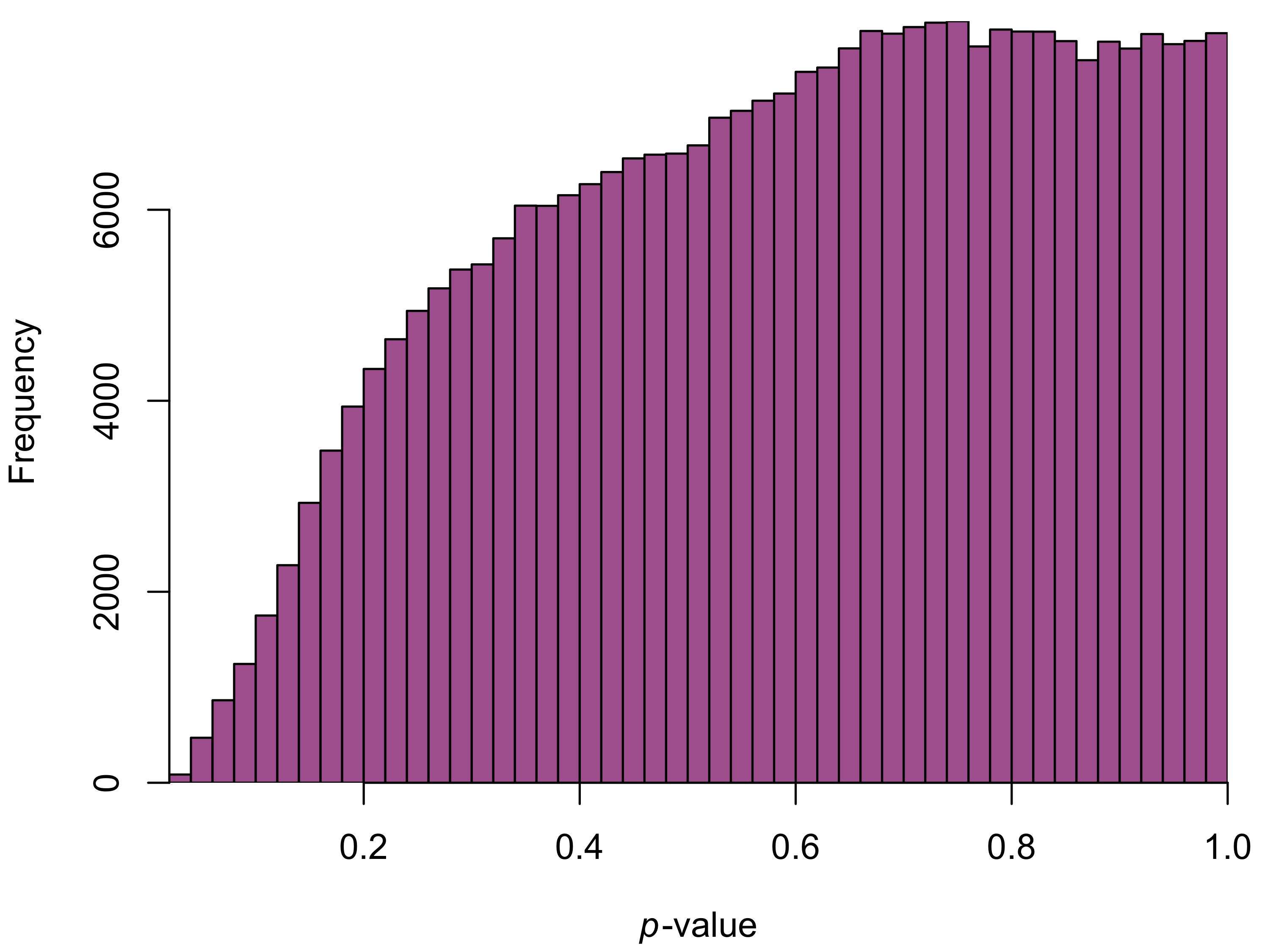
Unfortunately, the results aren’t quite what we wanted. While we’ve gotten rid of the huge peak on the left side of the histogram, we now have fewer small \(p\)-values than we’d expect by chance. ComBat seems to have over-corrected for the batches, leaving us with artificially small differences between the trilogies.
Even if the results aren’t perfect, they’re an improvement over the uncorrected values. The colour channel histograms show that the differences in colour spectrum have been reduced.
The most interesting part is to compare the screenshots themselves. The column on the left shows the original screenshot, with the right-hand side giving the ComBat-adjusted version.
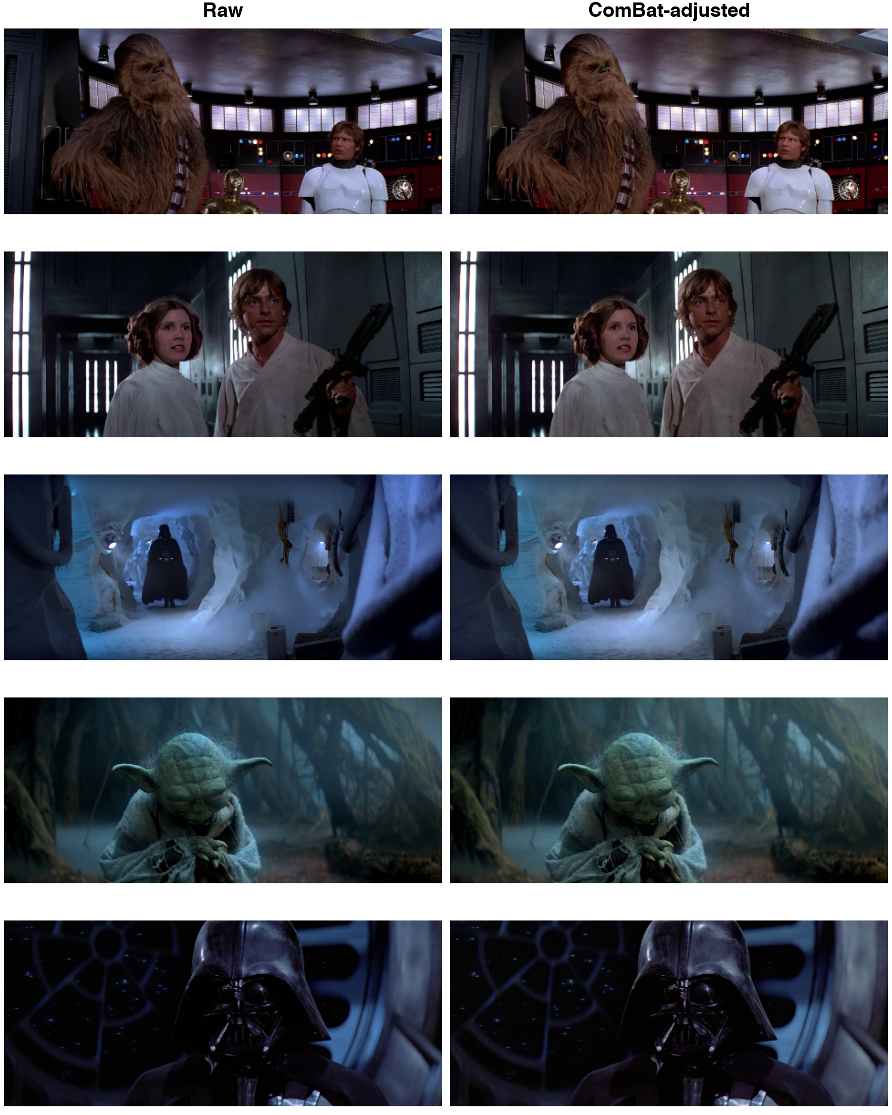
The screenshots above are all from the original trilogy, so we’d expect the ComBat-adjusted versions to have slightly warmer colours and less of a vignetting effect. The differences are subtle, but you can tell ComBat has made the window behind Darth Vadar brighter, for example.
Similarly, we can inspect the prequel trilogy. In these screenshots we’d expect ComBat to tone down the colours and add a vignetting effect.
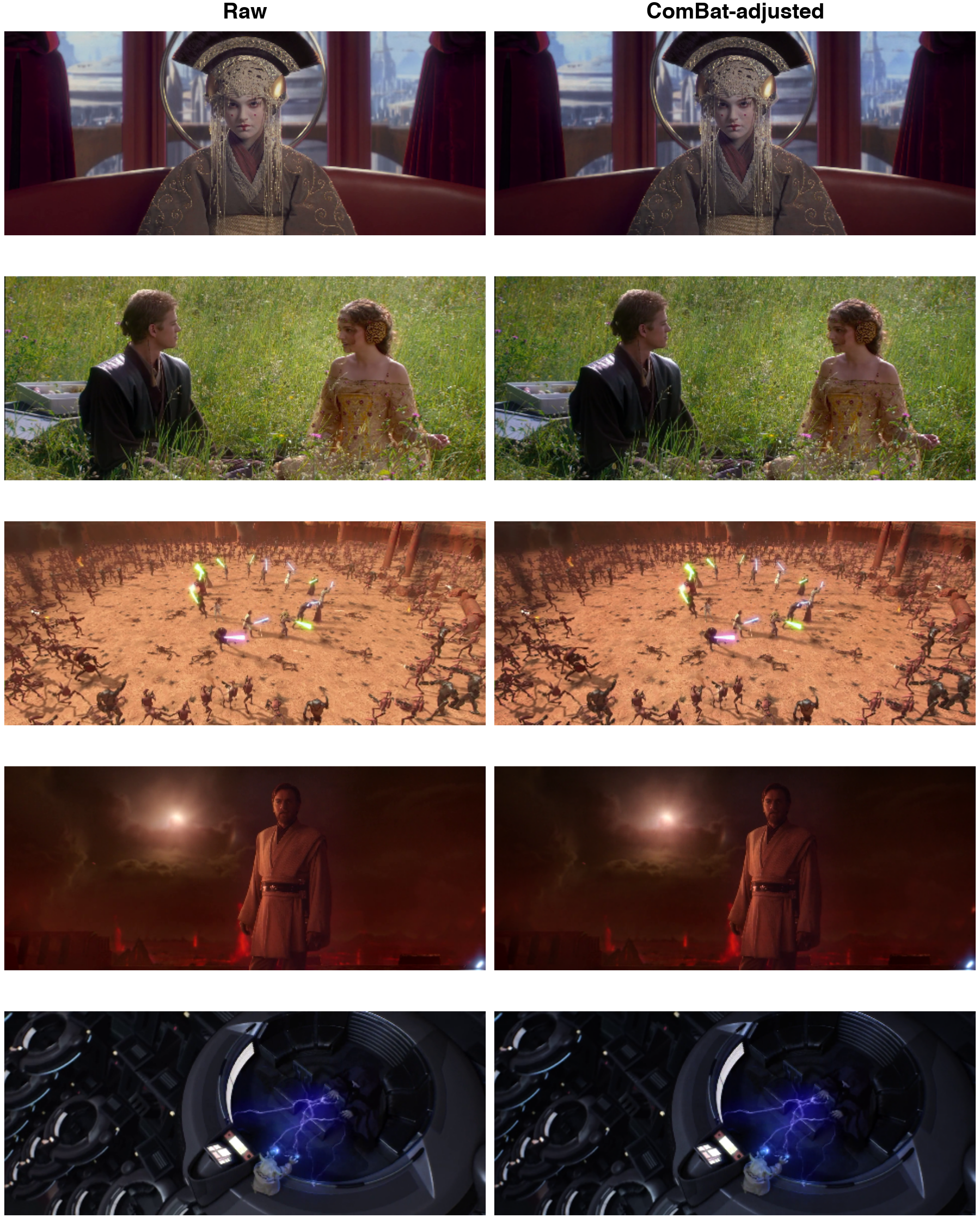
Like above, the differences are small. If I didn’t know what to look for, I’m not sure I’d see any at all. But the colours do seem to be darker in the ComBat-adjusted screenshots. For example, the grass behind Anakin and Padme is visibly darker after we’ve applied ComBat.
Conclusion
Unfortunately, I don’t think ComBat-adjustment of movies will go mainstream any time soon. I suspect modern video-editing has better ways of adding and removing vignetting, leaving my empirical Bayes approach as a largely academic exercise.
Even if you do want to run batch-correction methods from genomics on screenshots, there are better ways of doing it. For one thing, my analysis did not adjust for any covariates. To make sure we’re not removing genuine, biologically meaningful variation, we’d typically want to include relevant covariates in the model.
In Star Wars world, the most relevant covariate to adjust for would be where the plot takes place. Scenes in space are darker than scenes in the desert, and by including that information as a covariate we can make sure we’re not batch-adjusting for differences that stem from the plot itself.
Still, my naive, ComBat-approach worked better than I expected – and it was fun! On the off chance that you’d like to do something similar yourself, I’ve posted all of the code on GitHub.
References
Johnson, W. Evan, Cheng Li, and Ariel Rabinovic. “Adjusting batch effects in microarray expression data using empirical Bayes methods.” Biostatistics 8.1 (2007): 118-127.
Footnotes
The logit transform actually only makes sense for values in \((0, 1)\), so I used a trick from Stack Overflow to avoid all of my zeros and ones becoming NAs.↩︎
Of course, when you’re testing for batch effects there’s nothing “Hooray!” about a large number of significant results.↩︎
\(p\)-value histogram star David Robinson also has a great blogpost about empirical Bayes.↩︎