Bayesian extreme value models for tube delays
I have extremely mixed feelings about living in London. On the one hand, it’s an amazing city. There’s a never-ending list of attractions and neighbourhoods to explore. The tech scene is fantastic. A halloumi ice cream pop-up store opened in November.
On the other, there are the rental prices. The packed tubes. Single-glazed windows. My flatmates’ arguments over whether strategically placed liquor bottles are an adequate solution to our mouse problem.
Thursday, October 26th was one of those days when it didn’t seem worth it. Due to a signal failure at South Kensington, my usual forty-minute journey to work turned into an hour and forty minutes.
As I stood there, clinging to a strap on the District Line for an hour longer than usual, I started wondering how often I’ll have to put up with these delays. Thankfully I’m a statistician, and as I vaguely remembered from undergrad, there’s a whole branch of statistics dedicated to analyzing such questions.
Introduction to Extreme Value Theory
Extreme value theory is the study of statistical extremes. It’s best known as the statistics behind the (now-outdated) terms like “500-year-flood”, but it can be used to analyze extreme values in general.
Let \(X_1, X_2, ..., X_n\) be independent and identically distributed variables with a cumulative distribution function \(F\). Let \(M_n = \max \left(X_1, ..., X_n \right)\) denote their maximum value. By independence, we can express the distribution function \(G\) of the maximum as
\[\begin{equation} G(x) = P(M_n \leq x) = P(X_1 \leq x, ..., X_n \leq x) = F^n(x) \end{equation}\]
At this point, mathematical statistics starts to shine. The Fisher–Tippett–Gnedenko theorem states that as long as there exist normalizing constants \(a_n > 0\) and \(b\) and a distribution function \(H\) such that
\[\begin{equation} P \left( \frac{M_n - b_n}{a_n} \leq x \right) = F^n(a_nx + b_n) \rightarrow H(x) \end{equation}\]
then \(G(x)\) can only follow a generalized extreme value (GEV) distribution.
The generalized extreme value distribution is an extremely flexible distribution that encompasses the Weibull and Gumbel distributions as special cases. Its distribution function is given by
\[\begin{equation} F_{GEV}(z) = \exp \left( - \left( 1 + \frac{\xi(z - \mu)}{\sigma} \right)^{ -\frac{1}{\xi}}_p \right) \end{equation}\]
where \(x_p = \max(0, x)\) 1. The parameters \(\mu\), \(\sigma\), and \(\xi\) are the location, scale, and shape parameters, respectively.
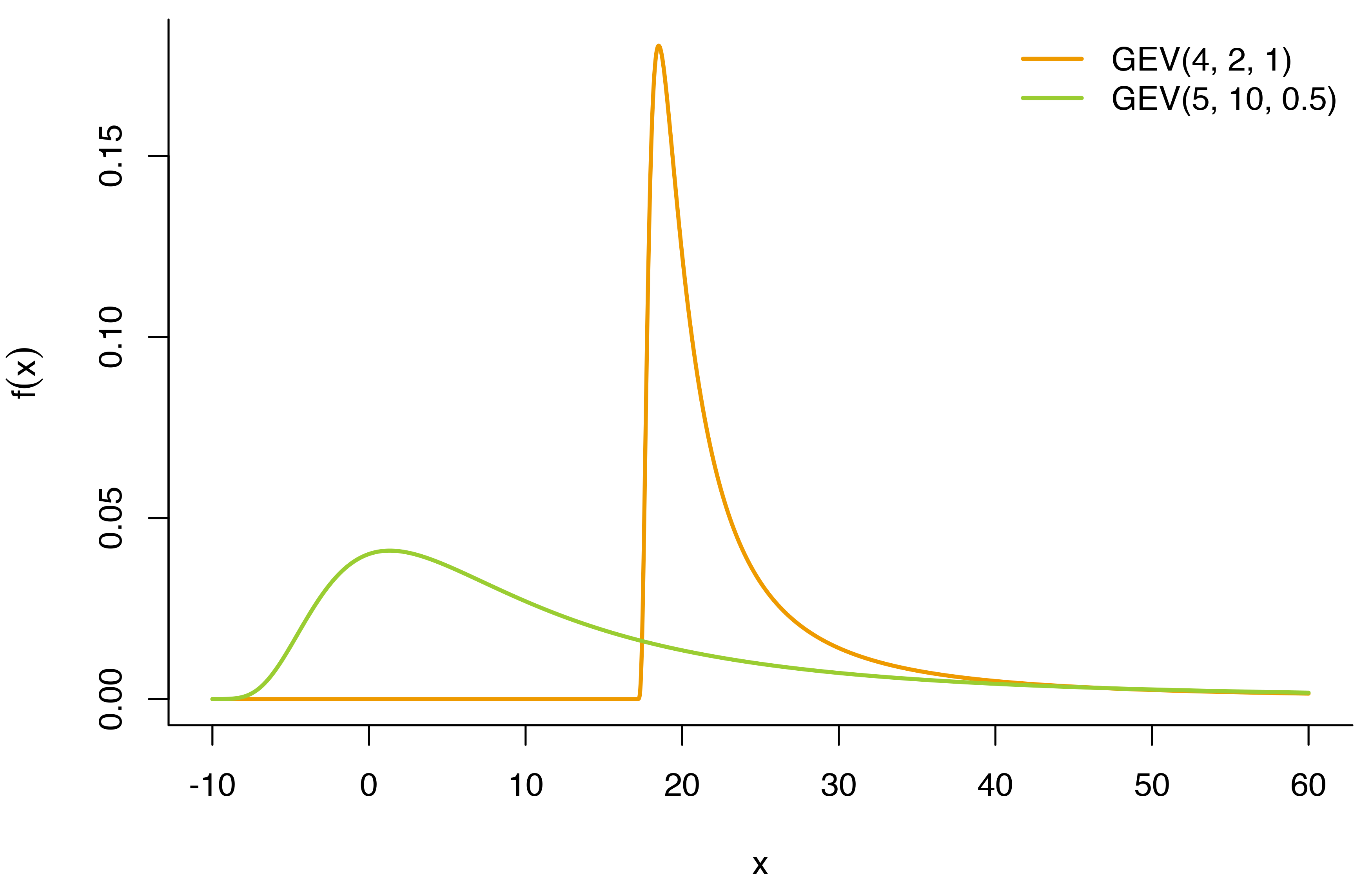
By the Fisher–Tippett–Gnedenko theorem, we know that (under some regularity conditions) our sequence of extreme values will follow a GEV distribution. This is true regardless of the underlying distribution of the data, which greatly limits the number of assumptions we have to make. Instead of deriving the distribution of the maximum from the distribution of the \(X_i\), we can focus on estimating the parameters \(\mu\), \(\sigma\), and \(\xi\) in the GEV distribution.
Direct Modelling of Journey Durations
Before fitting an extreme value model to my tube data, I wanted to try modelling the duration of my morning commute directly.
Transport for London lets you download the last eight weeks of data from your Oyster card. By the time I got around to doing this analysis, the October 26th data had disappeared from my history. I did however, experience another severe delay in early January. My tube was suspended, and I ended up walking from Westminster to South Kensington. I included this in the analysis by manually adjusting the row to include the full journey duration time (tube + foot) rather than only the Aldgate-Westminster portion of the journey.
The plot below shows the enter and exit times of all forty morning commutes included in my TfL history. Revealingly, you can tell I tend to get lazier as the week goes on and get in later on Thursdays and Fridays.
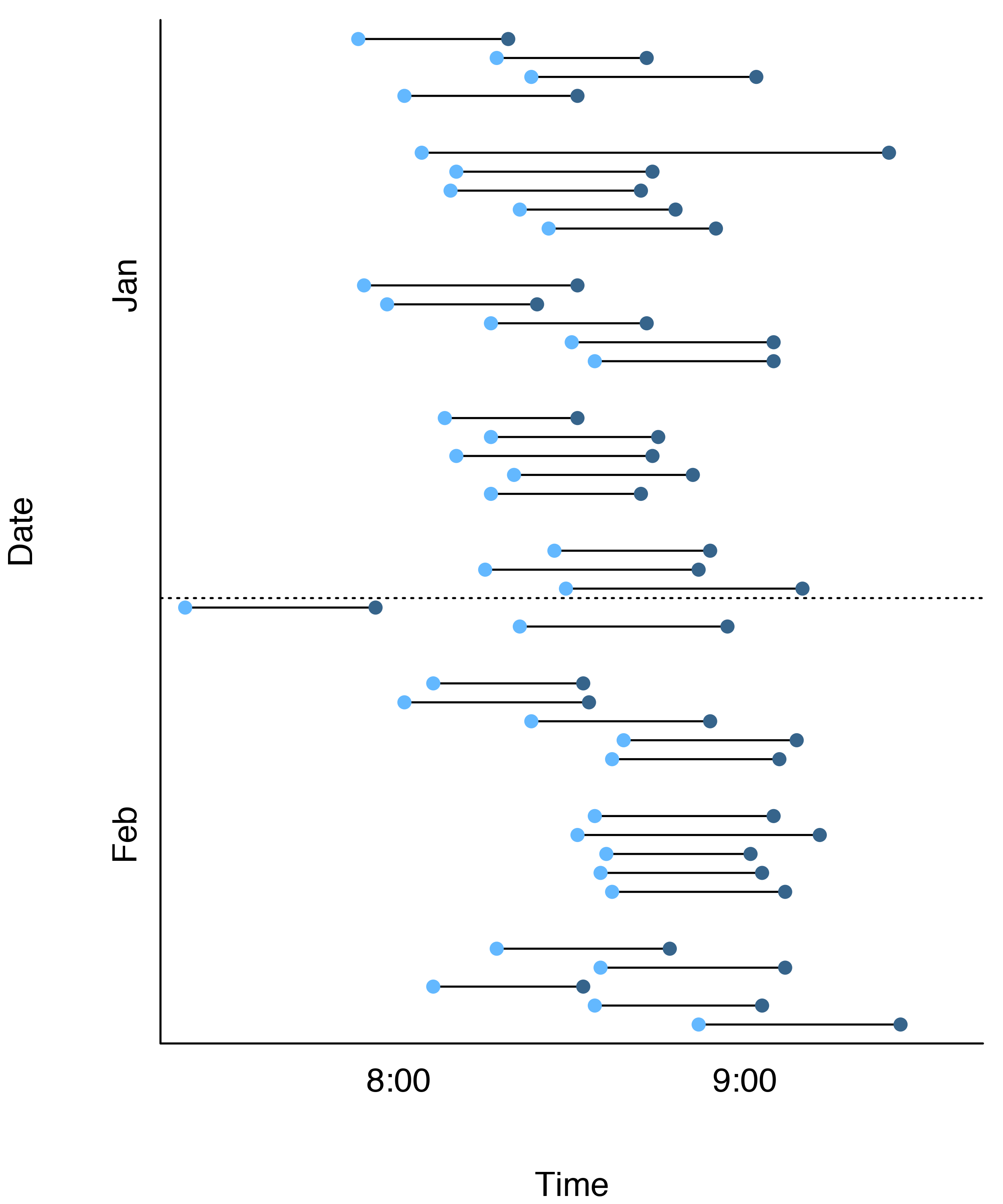
Even though 40 observations can be sufficient for a lot of analyses, it’s a tiny dataset in the context of extreme value modelling. Extreme values are rare by definition, and we’d typically like to have years worth of data to make sure we’ve observed an adequate number of them. To help with the data sparsity, I decided to go Bayesian.
Formulating a Prior
Unfortunately, Transport for London does not publish data on tube delays by line. The closest thing we have to historical data is a 5% sample of all journeys conducted during a week in November 2009, and I downloaded this data from the TfL website (account required).
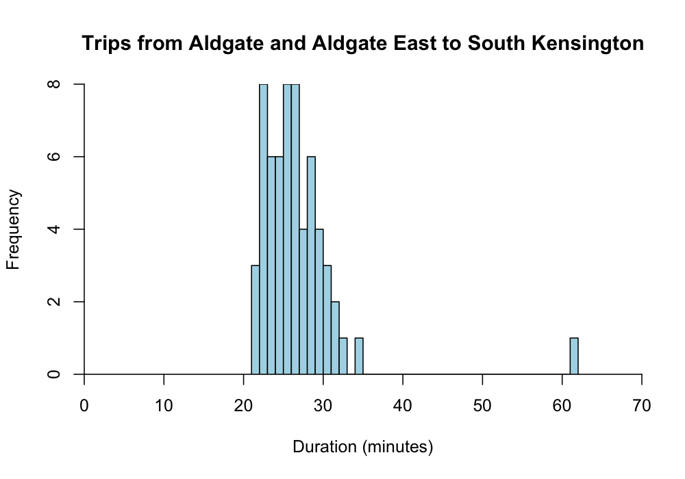
The dataset contains details of 2,623,487 tube journeys, 61 of which are between Aldgate or Aldgate East and South Kensington.2 As the histogram below shows, most of these journeys took between 20 and 30 minutes, with a single journey taking over an hour.
I used the truncated gamma distribution to model the journey durations. Transport for London currently lists the journey time from Aldgate East and Aldgate to South Kensington at 22 and 20 minutes, respectively, making it highly unlikely that my commute could be shorter than this. To account for the lower bound, I truncated the gamma distribution at 20 and assigned a probability of zero to all lower values.
truncated.gamma <- function(x, shape, rate, lower.truncation = 20) {

    # get density values without truncation
    raw.density <- ifelse(
        x > lower.truncation,
        dgamma(x, shape = shape, rate = rate),
        0
        );

    # divide by non-truncated area to obtain truncated density estimates
    truncated.area <- pgamma(lower.truncation, shape = shape, rate = rate);

    truncated.density <- raw.density/(1 - truncated.area);

    return(truncated.density);
}
After formulating the probability density function, I wrote a separate function for the log-likelihood of the model and used it to numerically obtain maximum likelihood estimates (MLEs) for the shape and rate parameters of the truncated gamma distribution.
truncated.gamma.loglik <- function(parameters, data) {
    shape <- parameters[1];
    rate <- parameters[2];

    loglik <- -sum( log(truncated.gamma(data, shape = shape, rate = rate)) );

    return(loglik);
}

optim.solution <- optim(
    par = c(1, 1), # initial values
    fn = truncated.gamma.loglik,
    data = durations
    );
The plot below shows the original histogram with the resulting, maximum likelihood-estimated truncated gamma distribution superimposed on the plot. The model seems to provide a reasonable fit to most of the data, although the observation at 60+ minutes could indicate that the true underlying distribution has a heavier tail. 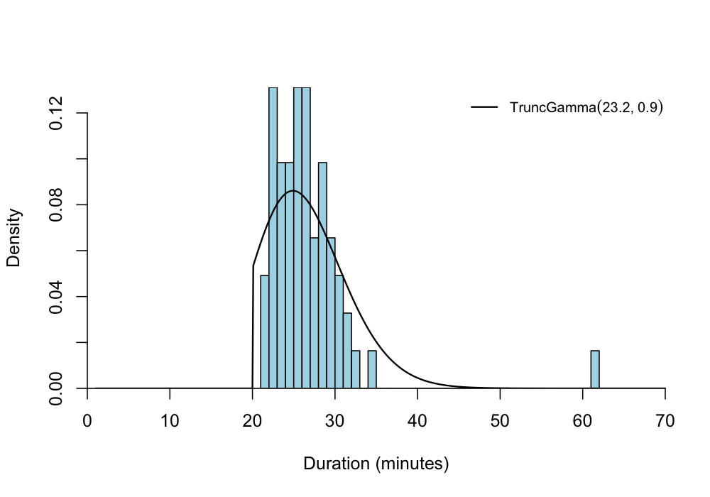
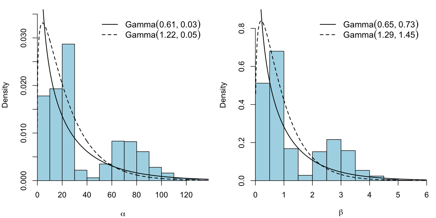
To incorporate these estimates into a prior distribution, we also need an estimate of the variability. I conducted a quick bootstrap study to get estimates for the variance of the MLEs of the shape and scale parameters, and matched these to gamma distributions.
\[\alpha \sim Gamma(0.61, 0.03)\] \[\beta \sim Gamma(0.65, 0.73)\]
When using historical data to calculate a prior distribution, a key question is how much weight to assign to the historical observations. Using the priors calculated above would be equivalent to weighing the historical data and new information equally - essentially a pooled meta-analysis. In my case, my own observations are more relevant than the historical observations. Traffic on the London Underground could have changed substantially since 2009, and not all of the historical observations were during the same time of day as my commute.
One way control the weight given to historical observations is through power priors. For gamma distributions, this means substituting a distribution \(Gamma(\alpha, \beta)\) for \(Gamma(\kappa\alpha, \kappa\beta)\). I decided on a somewhat arbitrary choice of \(\kappa = 2\), which corresponds to giving new observations twice the weight of historical data.
The plot below shows the \(\alpha\) and \(\beta\) values generated by each bootstrap simulation, the best fit Gamma distribution for each of them, and the power priors I opted for.
Stan Implementation
With the priors decided upon, I implemented the model in Stan. The T[] function provides an easy way of specifying truncated distributions. By adding it after a distribution declaration, you can truncate the distribution to the specified limits. For example, a ~ normal(0, 1) T[0,]; sets \(a\) to follow a standard normal distribution truncated to positive values.
data {
    int<lower=0> n;
    real<lower=0> y[n];
}

parameters {
    real<lower=0> alpha;
    real<lower=0> beta;
}

model {
    // prior distributions
    alpha ~ gamma(1.2161, 0.0524);
    beta ~ gamma(1.2946, 1.4505);

    for(i in 1:n)
        y[i] ~ gamma(alpha, beta) T[20,];
}
To fit the model I used the main workhorse function stan with four chains of length 2000, where the first 1000 iterations were used as a burn-in. One disadvantage of using truncated distributions is increased computational requirements – the MCMC sampling took around 20 minutes to run on my computer.
The histogram shows the observed morning commute times along with the posterior distribution of journey durations. In general the journey durations are longer than in the historical data, with a mean of around 30 minutes.
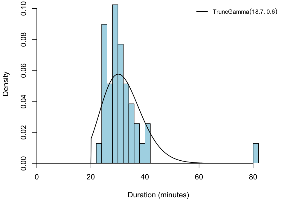
Even though the posterior distribution gives higher probabilities than the prior to journey times exceeding half an hour, the chances of extremely long journey durations are still very small. According to this model, the probability that my morning commute will take over an hour is \(6.01 \times 10^{-4}\). Assuming a five-day workweek, I can expect to spend over an hour to work about once every six and a half years. Considering I’ve experienced two such delays since October, that seems like an overly optimistic estimate.
Modelling via Generalized Extreme Value Distribution
So far we’ve been modelling the journey durations directly rather than the extreme values. For the extreme value analysis, I used the evdbayes package. There’s no vignette on CRAN, but if you download the package source code you will find a great user guide in the doc directory.
The package supports four different ways of constructing a prior (see section 4 of the user guide):
- Trivariate normal prior on \((\mu, \log \sigma, \xi)\)
- Trivariate normal prior on \((\log \mu, \log \sigma, \xi)\)
- Gamma distribution for quantile differences
- Beta distributions for probability ratios
In the interest of keeping things simple, I opted for the first approach. Modelling directly via the GEV distribution means we need to decide on a timeframe to take the maximum over. With only eight weeks of data it would be difficult to look at the monthly maximum, so I instead focused on modelling weekly maximum.
Conveniently, modelling the weekly maximum means we can use the 2009 TfL data to estimate a prior distribution. Section 6.1 of the evdbayes user guide shows an example of specifying a weak trivariate normal prior. I modified this example to incorporate the 2009 data. The longest journey duration during the week in November was 62 minutes, and I set this as the mean of the parameter \(\mu\). I also reduced the variance of \(\mu\) compared to the user guide (we have one data point as compared to their zero), but kept the priors for \(\sigma\) and \(\xi\) the same.
\[\mu \sim N(62, 10^3)\]
\[\log \sigma \sim N(0, 10^4)\]
\[\xi \sim N(0, 100)\]
The function prior.norm constructs the prior distribution, and the posterior function fits the model through MCMC. I used a run-length of 5000 and a burn-in of 1000 iterations. After running through it once, I experimented with different initial values to make sure my results weren’t unduly affected by the starting points of the chain.
cov.matrix <- diag(c(1000, 10000, 100))
prior <- prior.norm(
    mean = c(62, 0, 0),
    cov = cov.matrix
    );

mcmc.result <- posterior(
    n = 5000,
    burn = 1000,
    init = c(10, 10, 10),
    prior = prior,
    lh = 'gev',
    data = weekly.max$duration,
    psd = c(0.5, 0.5, 0.5)
    );
The histograms below show the values of the parameters over the 4000 MCMC samples. These seem robust to the initial settings of the chain, indicating that the MCMC algorithm has converged.
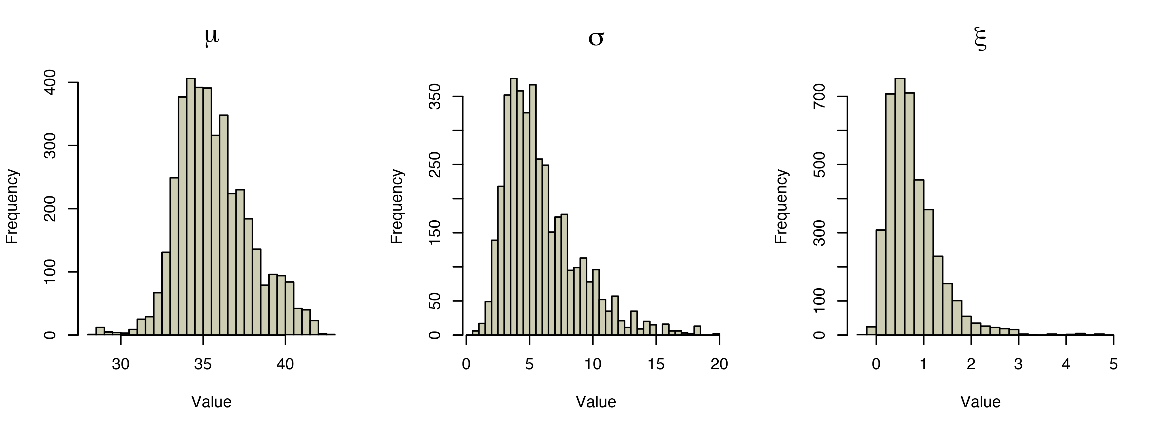
We take the posterior mean of each of these distributions as our parameter estimates \(\hat{\mu} = 35.7, \hat{\sigma} = 5.9\), and \(\hat{\xi} = 0.77\). The resulting generalized extreme value distribution is shown below, with the black dots showing the observed weekly maxima. The density function increases sharply between 30 and 35 minutes before starting to decrease into a heavy right tail.
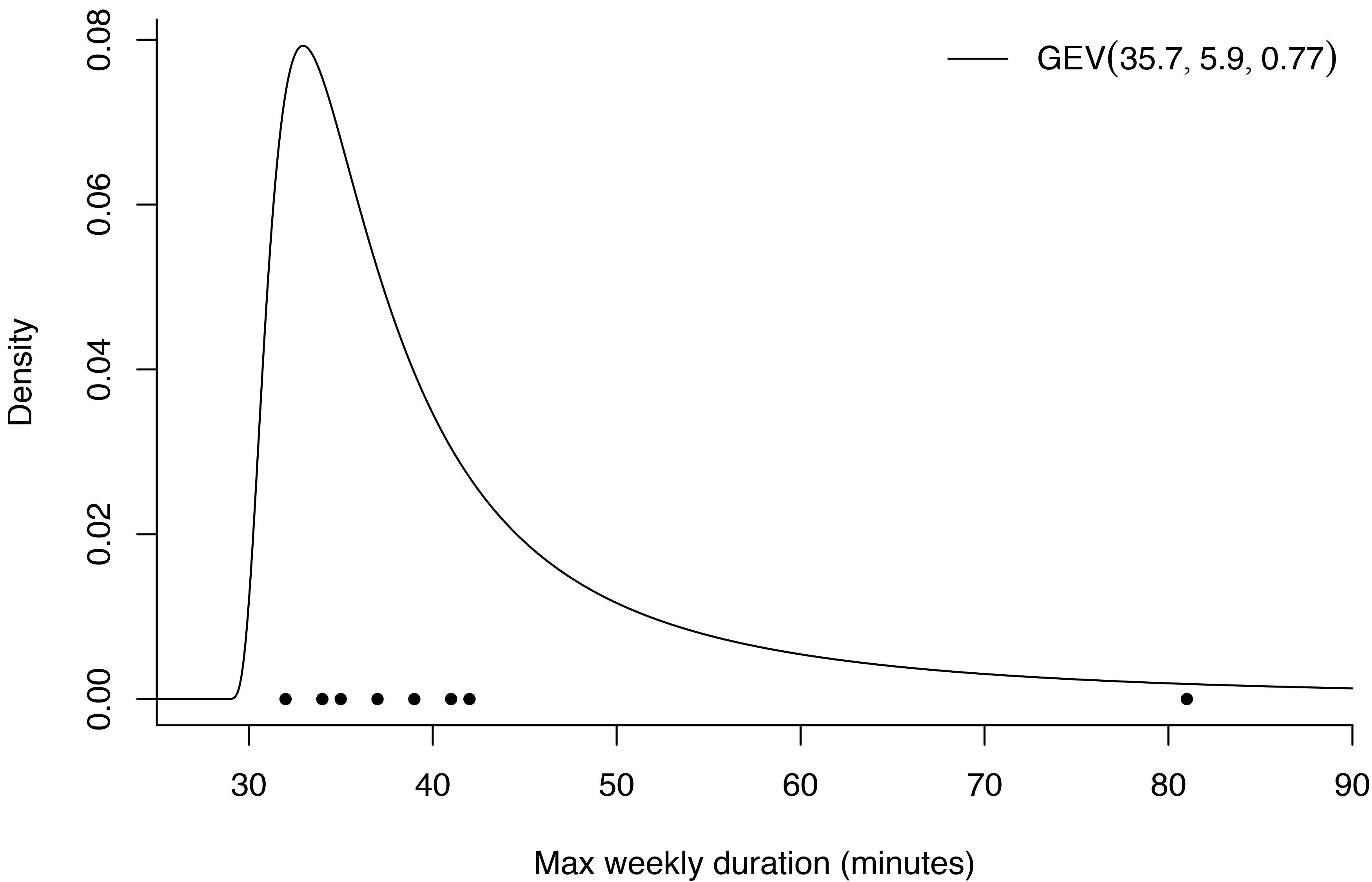
According to this posterior distribution, there is a roughly 15% chance that my longest commute in a week will take longer than an hour. In other words, I should expect a delay this severe every seven weeks or so. Even less encouraging, there’s a 6% chance of the weekly maximum exceeding 90 minutes. If the model is correct, I can expect to feel very frustrated with London every three to four months.
| Duration | Truncated gamma model expected frequency | GEV model expected frequency |
|---|---|---|
| >60 minutes | Every 6.4 years | Every 6.9 weeks |
| >90 minutes | Every 411,313 years | Every 3.6 months |
By contrast, the truncated gamma model for commute duration expects a 90 minute journey to occur only once every 411,313 years! The large differences are most likely the result of the truncatad gamma model not providing a good fit to the longest commute times. Even if the model fits well for the bulk of the observations, it does not seem to work for the tails. By using the Fisher–Tippett–Gnedenko theorem, we’re able to model the extremes even when we don’t have a good model for the underlying data.
Conclusion
Tube delays are likely to remain one of my recurring complaints about London, but there are few silver linings. For one thing, housing and commuting never grow old as conversation topics with Londoners. And for another, recurrent delays can be an excuse to get creative with extreme value models!
References
Congdon, Peter. Applied bayesian modelling. Vol. 595. John Wiley & Sons, 2014.
De Haan, Laurens, and Ana Ferreira. Extreme value theory: an introduction. Springer Science & Business Media, 2007.
Lunn, David, et al. The BUGS book: A practical introduction to Bayesian analysis. CRC press, 2012.